Power Query lets you perform a series of steps to transform your Excel data. There are times when we want to do things that are not built in the user interface. This is possible with Power Query’s programming language, which is M.
Unfortunately not all of Excel’s formulas can be used in M.
For example, if we want to use the LEFT Excel Function, it is not supported in M.
But I have found a way for us to replicate the LEFT Function in M!
Table of Contents
Step By Step Guide
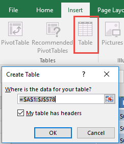
STEP 1: Select your data and turn it into an Excel Table by pressing the shortcut Ctrl + T or by going to Insert > Table
STEP 2: Go to Data > Get & Transform > From Table (Excel 2016) or Power Query > Excel Data > From Table (Excel 2013 & 2010)
Excel 2016:
Excel 2013 & 2010:
STEP 3: This will open up the Power Query Editor.
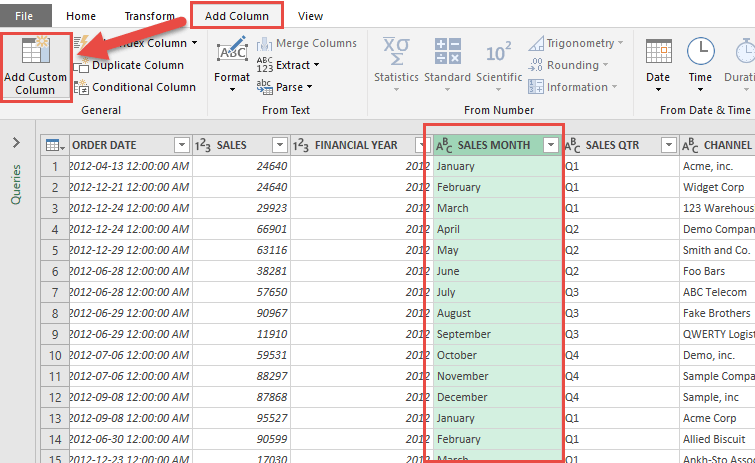
Go to Add Column > Add Custom Column
We want to get the first 3 characters of the Sales Month:
STEP 4: Let us create a simple M expression to replicate the LEFT function in Excel.
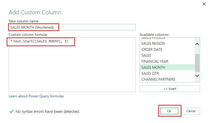
In the New column name text box, type SALES MONTH (Shortened)
In the Custom column formula, type in: Text.Start(
From the Available columns choose SALES MONTH and Insert
Then finish off the formula by entering , 3)
We now have build the following formula:
Text.Start([SALES MONTH], 3)
So lets quickly break down what we just did:
- We are using the Text.Start formula to get the first X characters of the SALES MONTH column
- We place in 3, to specify that we want the first 3 characters.
Click OK to confirm.
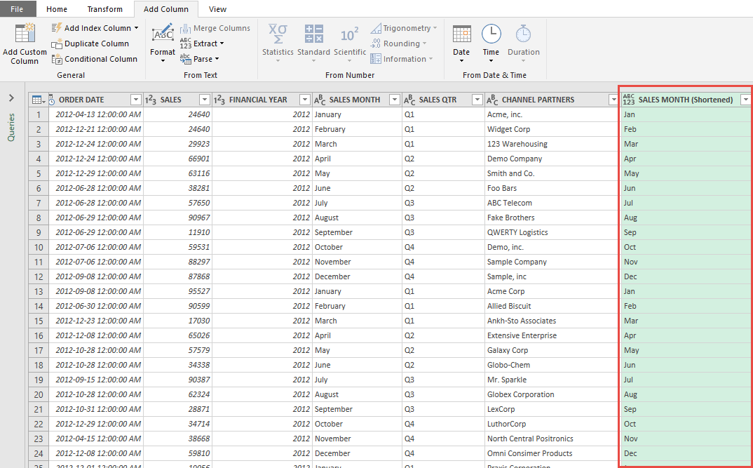
Now you will see your changes take place.
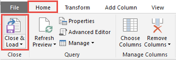
STEP 5: Click Close & Load from the Home tab and this will open up a brand new worksheet in your Excel workbook with the updated values.
Congratulations! You have used a M formula for replicating the LEFT function!
Conclusion
Further Learning:
- Replicating Excel’s RIGHT Function with M in Power Query
- Replicating Excel’s FIND Function with M in Power Query
- Replicating Excel’s LEN Function with M in Power Query
Bryan
Bryan is a best-selling book author of the 101 Excel Series paperback books.
