You can easily Excel find last value in column using the OFFSET function.
Just follow the tutorial below and you can fetch that last value. But before you move, let’s first understand how the OFFSET function works!
What does it do?
It returns a reference to a range, from a starting point to a specified number of rows, columns, height, and width of cells
Formula breakdown:
=OFFSET(reference, rows, columns, [height], [width])
What it means:
- reference – It is the starting point from which you want to base the offset function. Required
- rows – It is the number of cells you want to go up/down. Required
- columns – It is the number of cells you want to go left/right. Required
- height – It is the number of rows you want the return reference to be. Optional
- width – It is the number of columns you want the return reference to be. Optional
If you omit the height or width argument, the output will have the same height or width as a reference!
The OFFSET function in Excel is one of the Lookup functions and is great if you want to reference a range of cells and use that reference to do a calculation.
Click here to see how the formula works visually & interactively!
Now that you are familiar with offset function, let’s see how excel return last value in column!
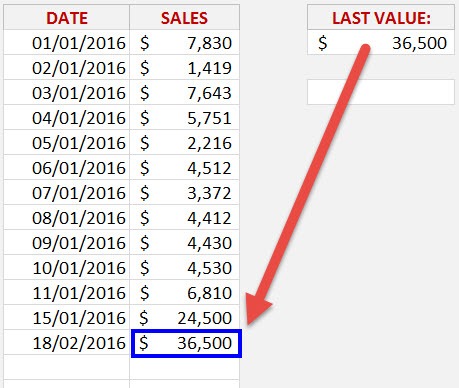
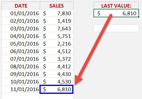
In this example, we have a list that we enter our daily sales into and want to show the last transactional value entered.
This can be used to highlight the latest sales value in a Dashboard or daily metrics report.
Watch it on YouTube and give it a thumbs-up!
Follow the step-by-step tutorial on Excel find last value in column and download this Excel workbook to practice along:
STEP 1: We need to enter the Offset function
Table of Contents
=OFFSET
STEP 2: 1st Offset argument – Where do we want to start our reference?
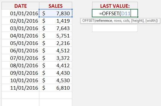
This is at the start of the Daily Sales list:
=OFFSET(D11
STEP 3: 2nd Offset argument – How many Rows down do we want to go?
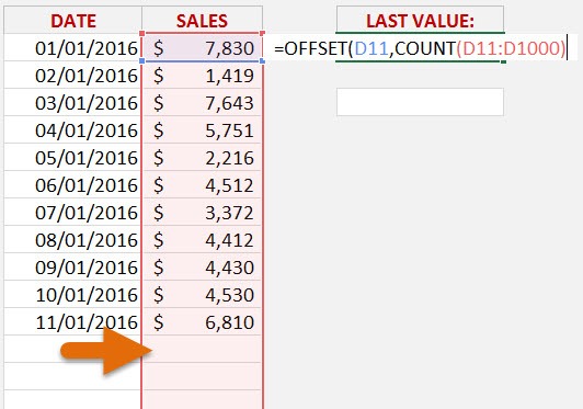
This is where the COUNT function is used to count how many transactions we have in our list and go down by that amount.
So as we are starting at cell D11, we are going to go down 11 cells ( COUNTA(D11:D1000) ) and we end up after the last cell with a value.
NB: It is always a good idea to enter an ending range that is more than your last data cell. That way as your new data get entered, we will be sure to capture it!
=OFFSET(D11, COUNT(D11:D1000)
STEP 4: How many of the last sales transactions do we want to Sum? 1
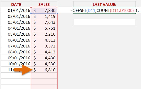
So we need to take away 1 from the COUNT formula which means that our Offset function will go up by 1 cell:
=OFFSET(D11, COUNT(D11:D1000)-1,
STEP 5: 3rd Offset argument – How many Columns to the right/left do we want to move?
We do not want to move to any Columns, so we simply enter 0
=OFFSET(D11, COUNT(D11:D1000)-1,0,
STEP 6: 4th Offset argument – How High do we want our referenced data to be?
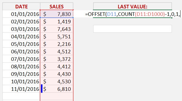
Since we want to show the last transaction, then we need the [height] to be 1 cell high:
=OFFSET(D11, COUNT(D11:D1000)-1,0,1,
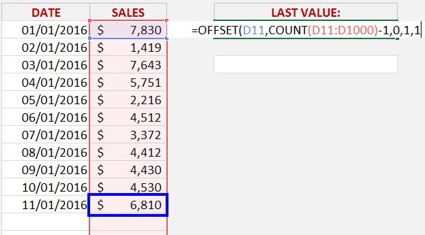
STEP 7: 5th Offset argument – How Wide do we want our referenced data to be?
We want to reference 1 Column only, so we need to enter 1 for the [width]
=OFFSET(D11, COUNT(D11:D1000)-1,0,1,1))
As we can see the Sum of the last transaction from our example is $6,810.
This is how you can use Excel formula last cell in column with data!
This formula is dynamic as well. If we add more transactions at the bottom of our Sales list then it automatically Excel find last value in column, without the need to update the formula 🙂
Let’s try that!
In this example, you have added two additional daily sales data and you will see the value returned by the formula will be updated.
This completes our Excel last value in column using the OFFSET function!
Make sure to download our FREE PDF on the 333 Excel keyboard Shortcuts here:
John Michaloudis is a former accountant and finance analyst at General Electric, a Microsoft MVP since 2020, an Amazon #1 bestselling author of 4 Microsoft Excel books and teacher of Microsoft Excel & Office over at his flagship Academy Online Course.
