– Performing calculations or analysis on the date and time components separately.
– Formatting the date and time differently for presentation or reporting.
– Integrating date and time data into other applications or systems that require them to be separate.
In this article, we will explore various methods to separate date and time in Excel –
Download the Excel Workbook below to follow along and understand How to Separate Date and Time in Excel –
download excel workbookSeparateDateandTime.xlsx
Text to Columns
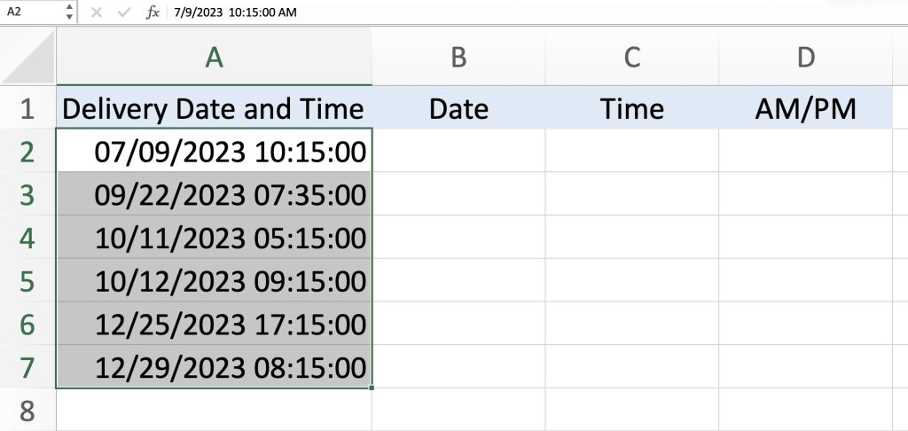
Select the cell or column containing the combined date and time data.
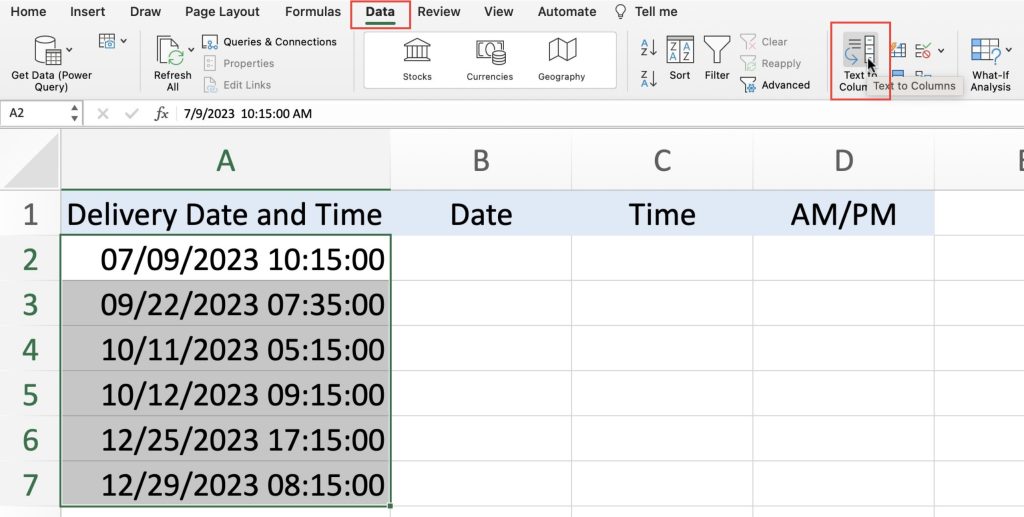
Go to the Data tab and click on Text to Columns.
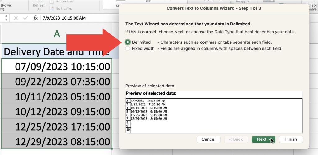
Choose Delimited in the wizard then select Next.
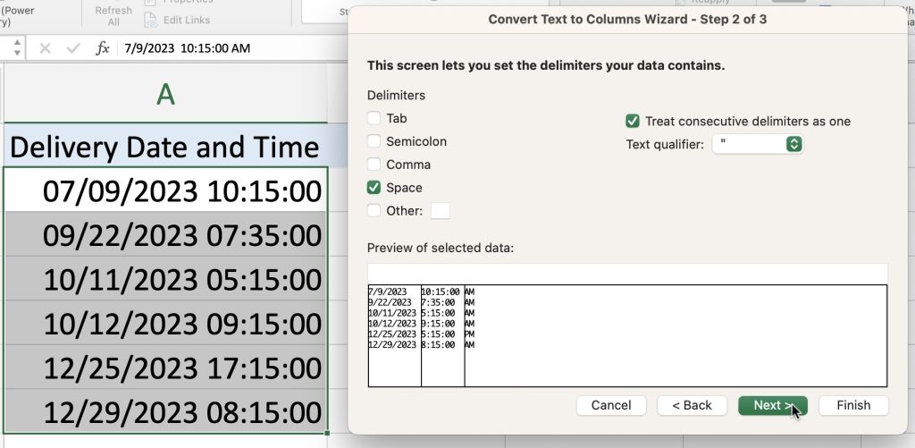
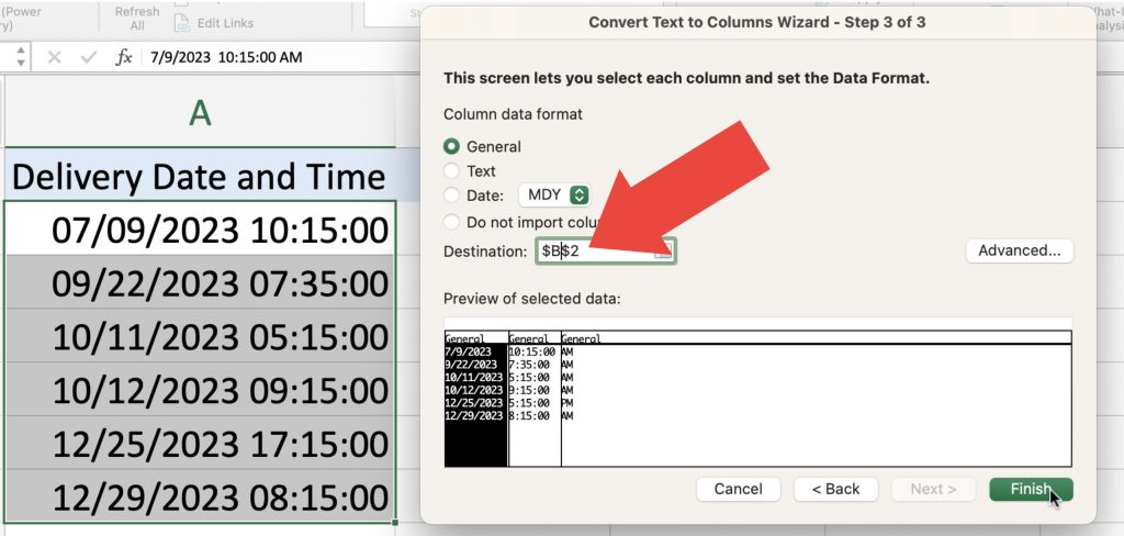
Select the appropriate delimiter that separates date and time (e.g., space or a comma). In our case we will select Space, then click Next.
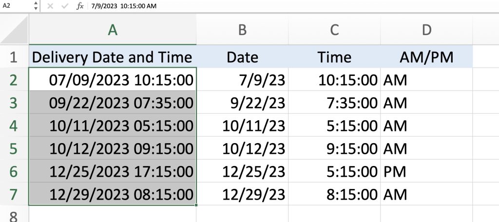
From here, we need to decide where we want the split data times to appear. By default it will overwrite the existing values. But we can change it to C2 instead.
Click Finish.
Click here to learn how to Split First & Last Name Using Text to Columns!
LEFT and RIGHT Functions
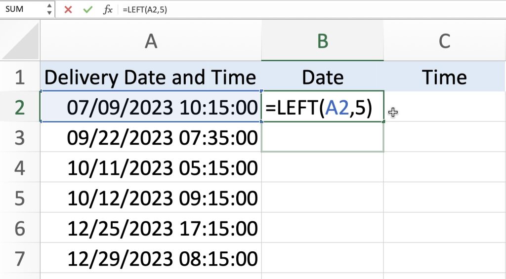
You can use the LEFT and RIGHT functions to extract specific portions of text data. Assuming the date is on the left side of the combined data, you can use the LEFT function to extract it to column B.
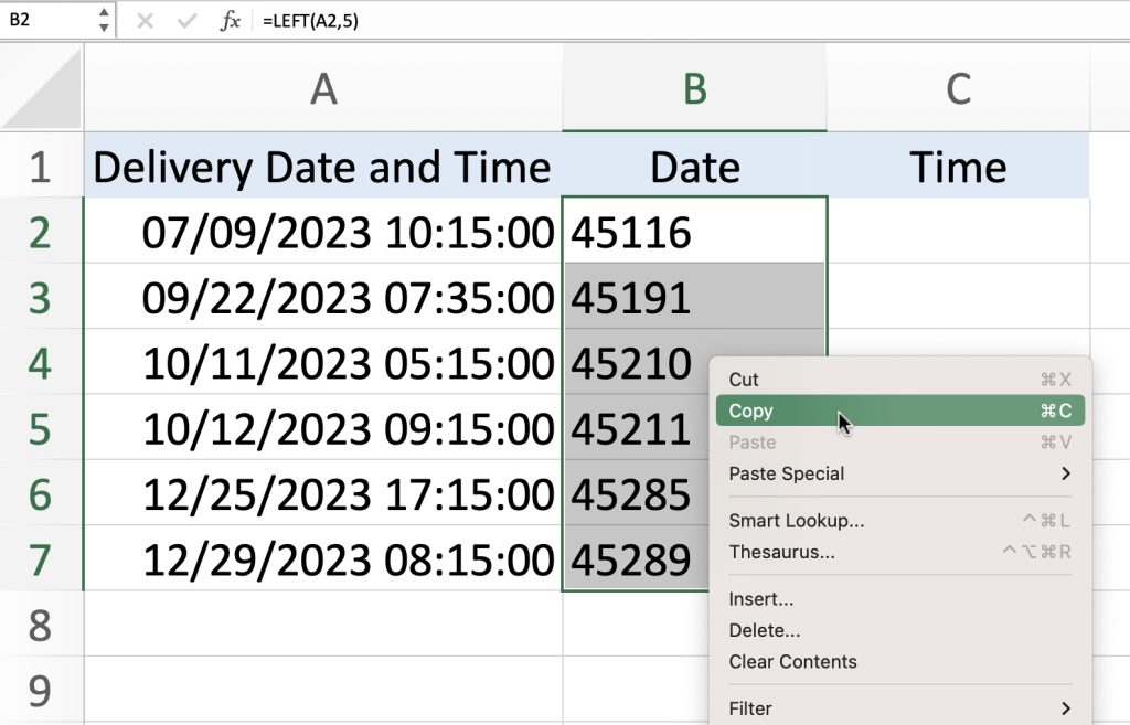
In cell B2, enter =LEFT(A2,5)
(The number 5 represents the number of characters removed from the right. Essentially, only leaving the date value)
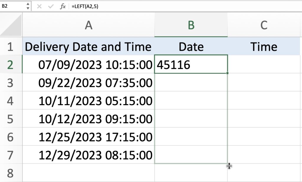
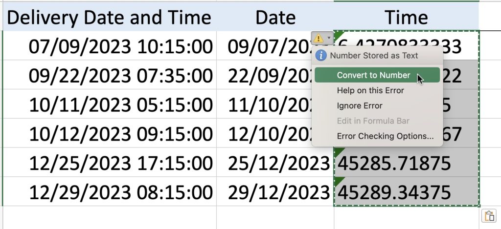
As you can see the data comes out in a different code. Before we can change this into a date format, we will drag the formula all the way down to the bottom of the column.
Highlight the cells in column B, right-click, select Copy.
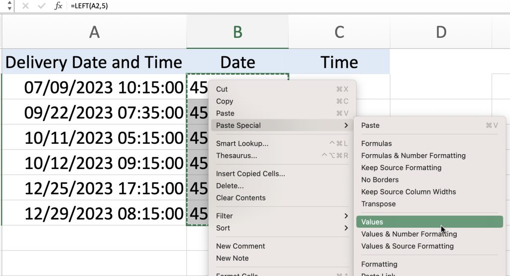
Right-click again, and select Paste by Value.
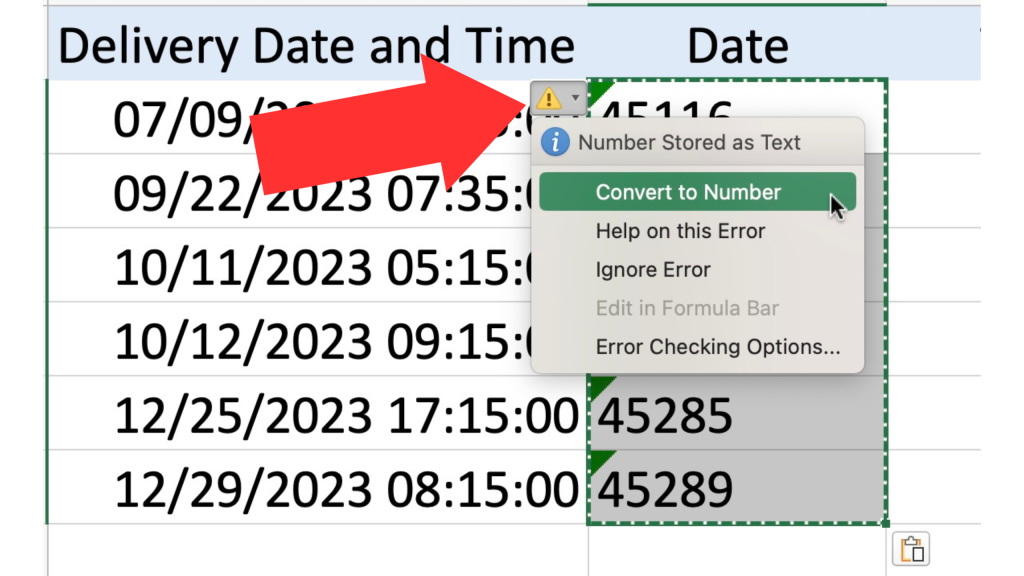
Click on the caution box, and select Convert to Numbers.
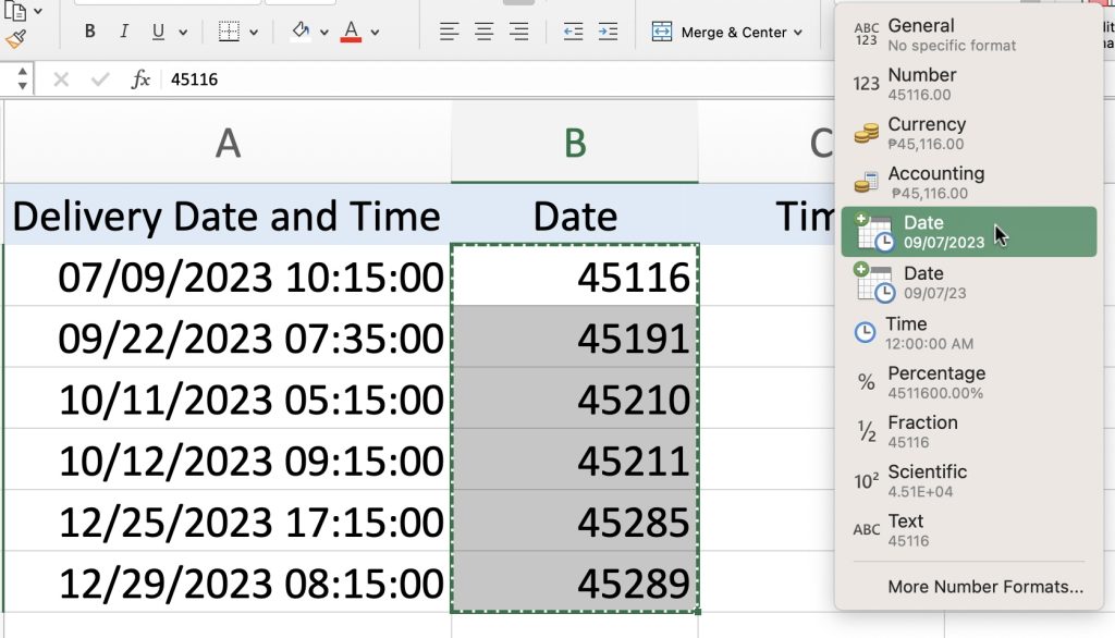
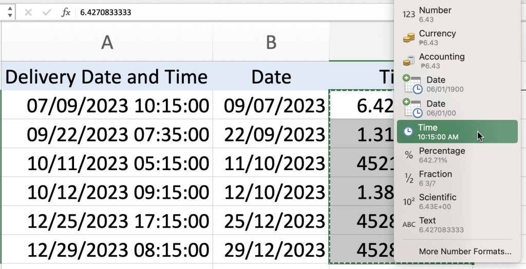
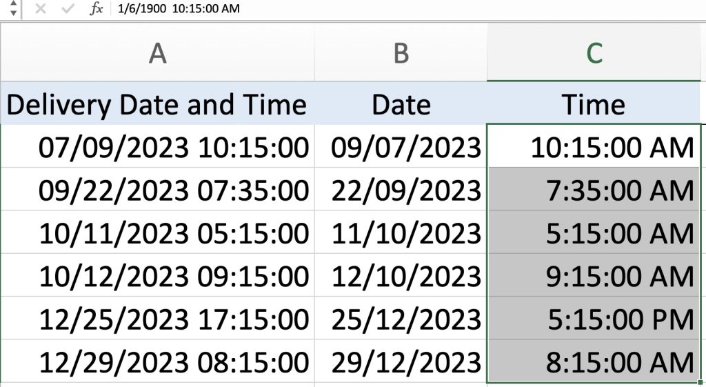
Right-click and select Format Cells. Select Date. Click OK.
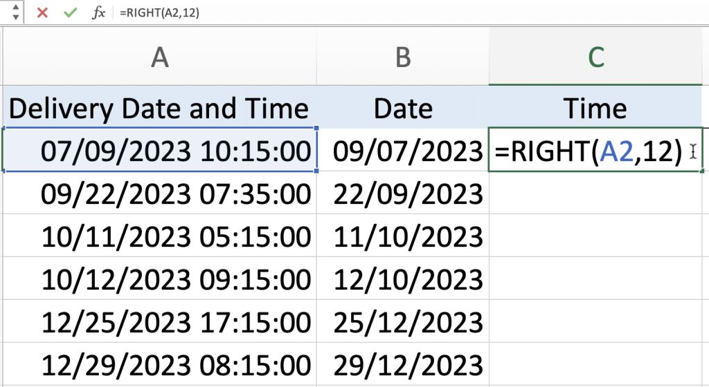
To extract the time, you can use RIGHT function. Assuming the time is on the right side of the combined data, you can use the RIGHT function to extract it to column C.
In cell C2, enter =RIGHT(A2,12)
(The number 12 represents the number of characters removed from the right. Essentially, only leaving the time value)
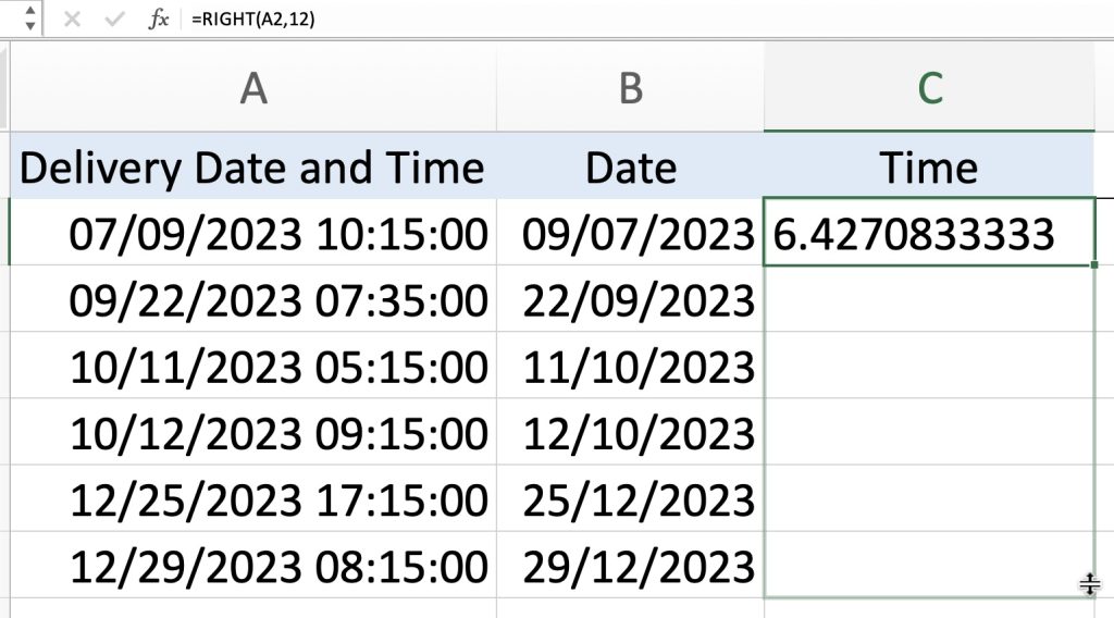
As you can see the data comes out in a different code. Before we can change this into a date format, we will drag the formula all the way down to the bottom of the column.
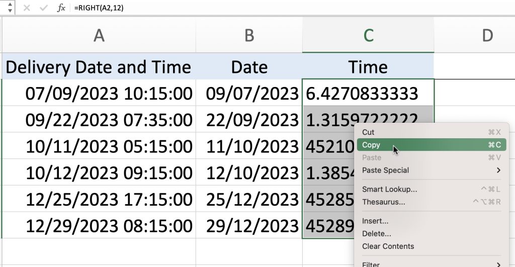
Highlight the cells in column C, right-click, select Copy.
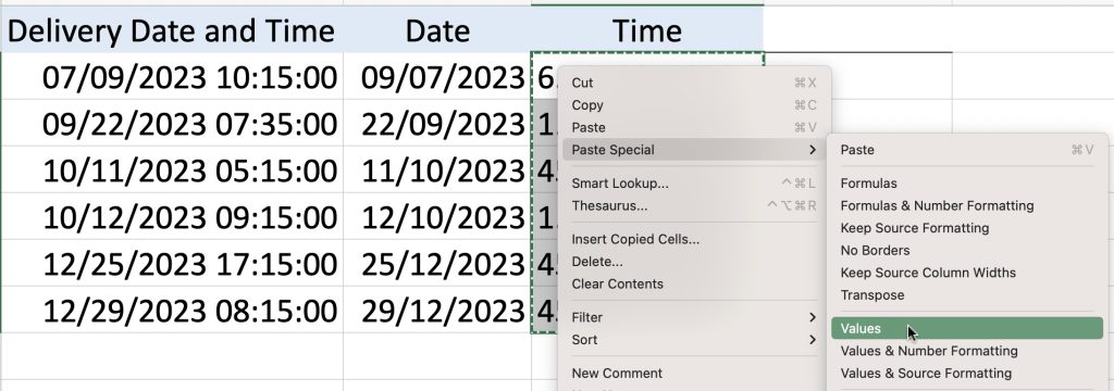
Right-click again, and select Paste by Value.
Click on the caution box, and select Convert to Numbers.
Right-click and select Format Cells. Select Time. Click OK.
Click here to Unlock the Power of Excel: 8 Substring Functions for Easy Data Analysis
INT and MOD Functions
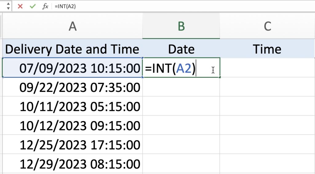
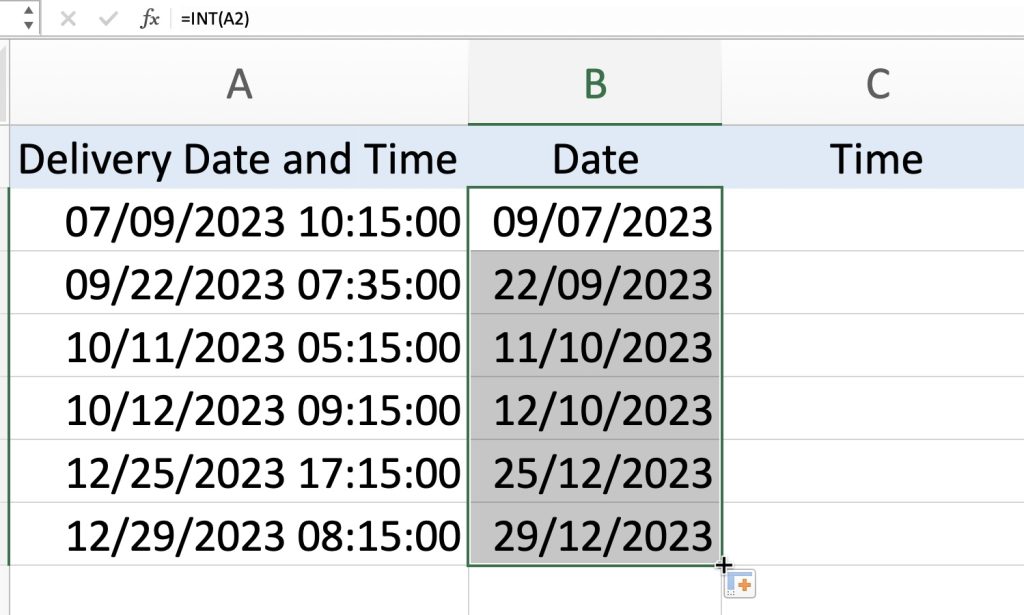
Let’s say we have the date and time values in Column A. To get the date portion, we can use the INT function.
In cell B2, enter =INT(A2)
Double-click or click and drag the small square on the bottom-right corner of cell B2 to apply the formula to the rest of the column.
(You may notice that the format is still showing the time as 00:00:00. To remove this, right-click and select Format Cell. Select Date.)
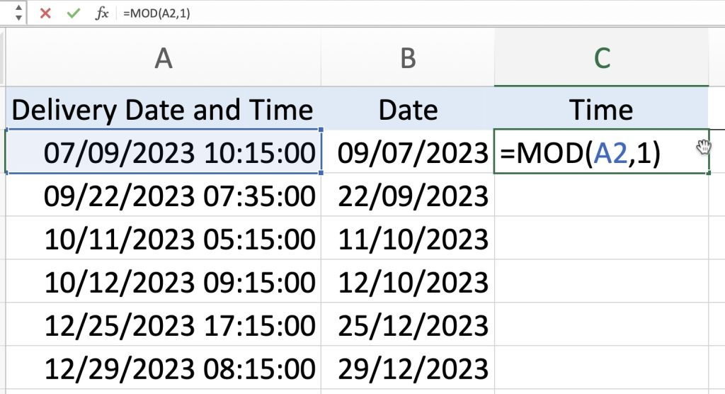
To get the time element, we can use the MOD function. click on cell C2, and enter =MOD(A2,1)
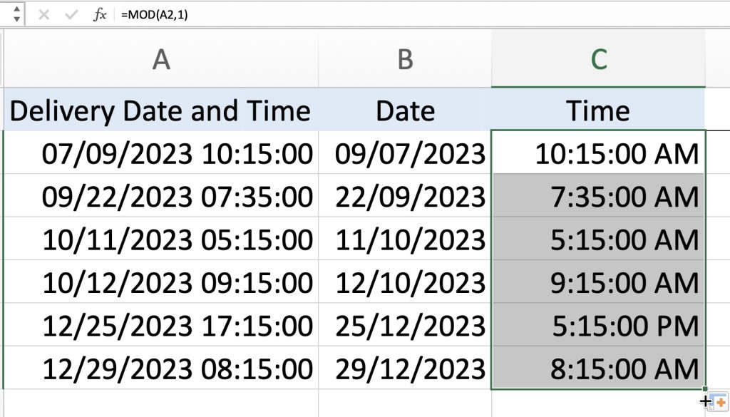
Double-click or click and drag the small square on the bottom-right corner of cell B2 to apply the formula to the rest of the column.
(The format will may show the date. Right-click and click on Format Cell. Choose Time.)
Click here to learn How to get Remainder in Excel using MOD Formula!
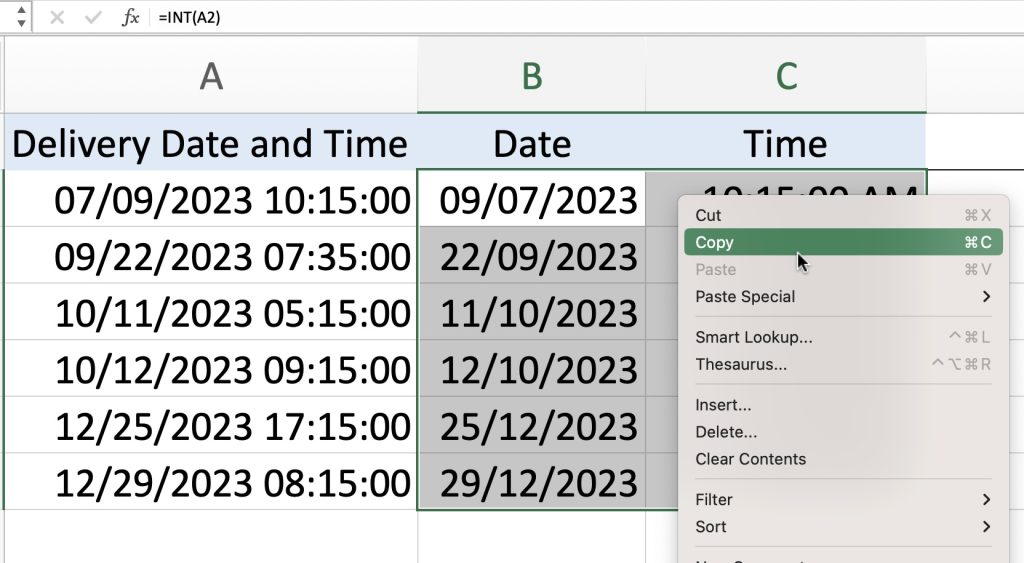
By default, these formulas will be linked to the original values. If you change the values in Column A, it will directly reflect the changes in Column B and C. The formula is dynamic.
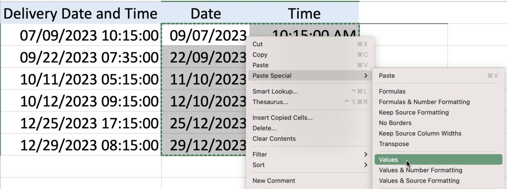
If you want Columns B and C to be independent of Column A, highlight B2 to C7. Right-click and Copy. Right-click again, and select Paste Values.
Power Query
Power Query is a powerful data transformation tool available in Excel. It can be used to split and manipulate date and time data with ease. You can use the Split Column feature to divide the data based on specific criteria.
Select Column A
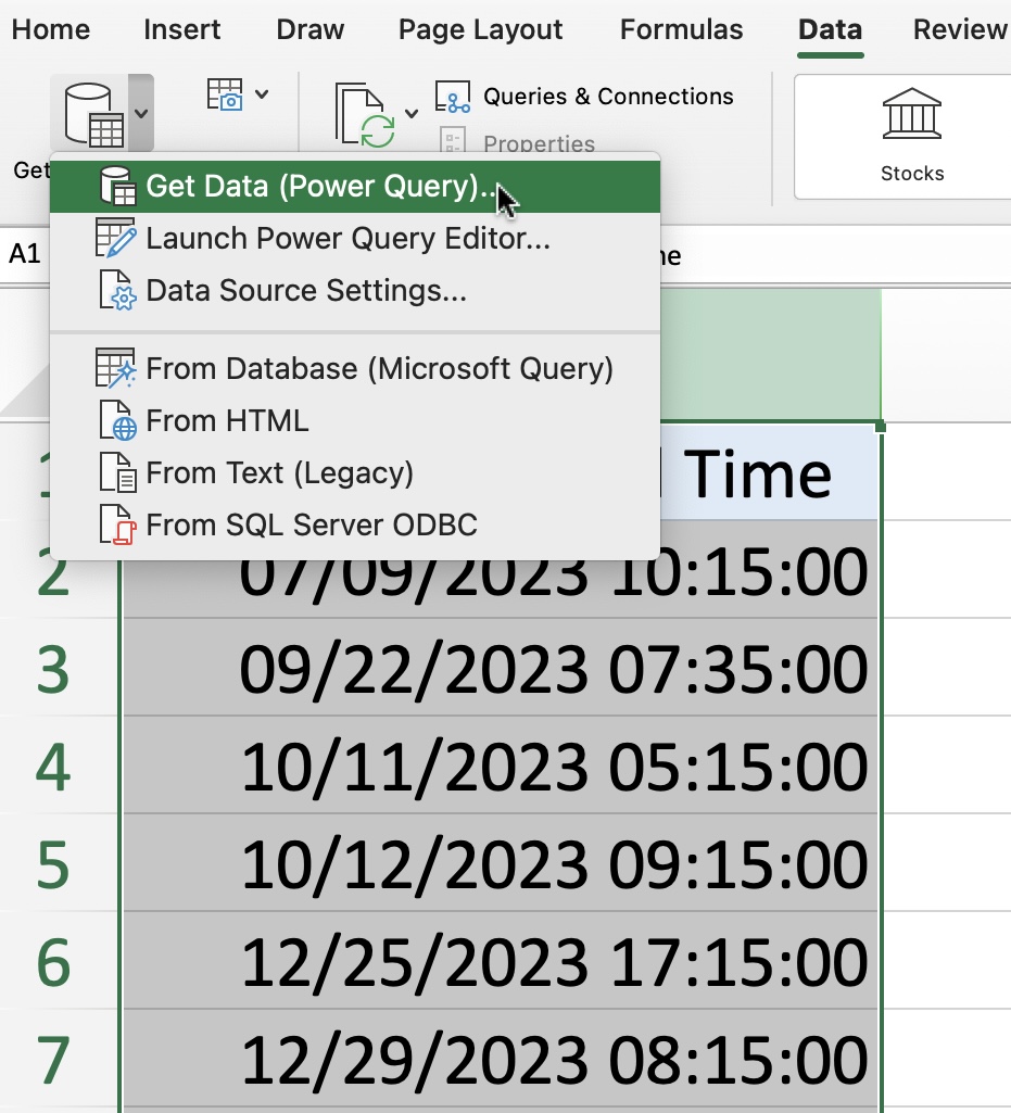
Go to the Data tab and click on Get Data or Get & Transform Data.
Click on From Sheet.
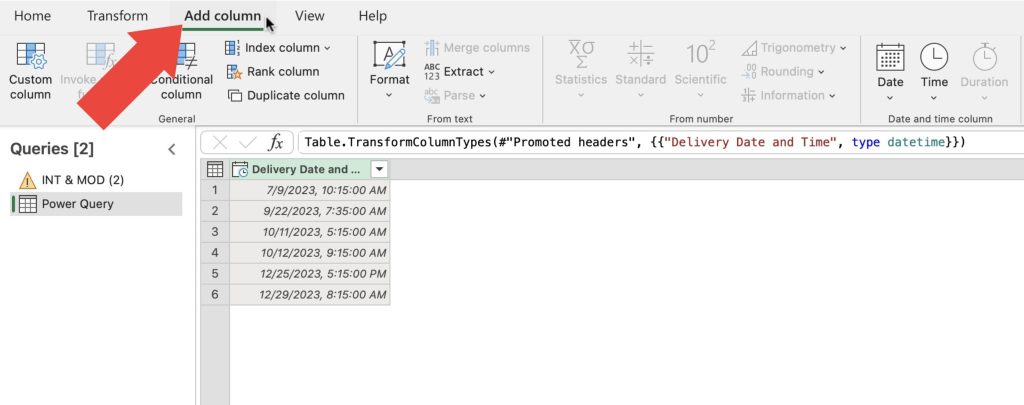
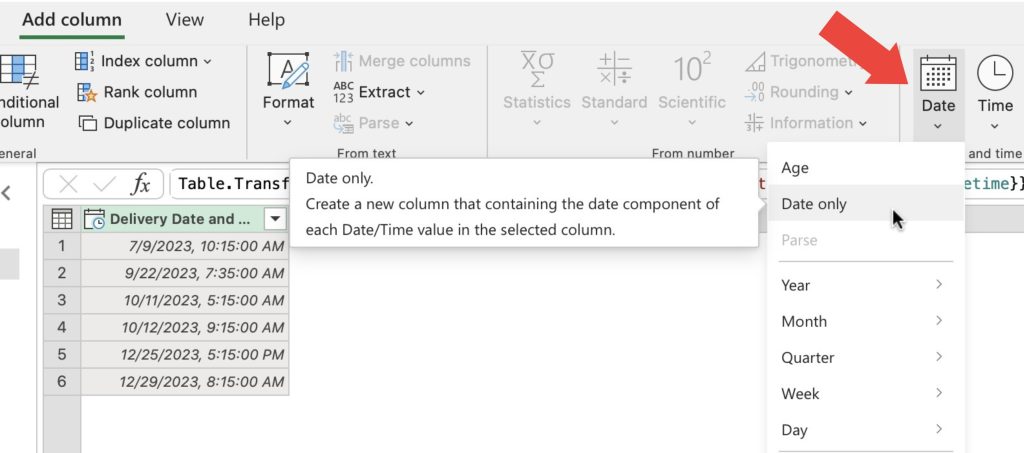
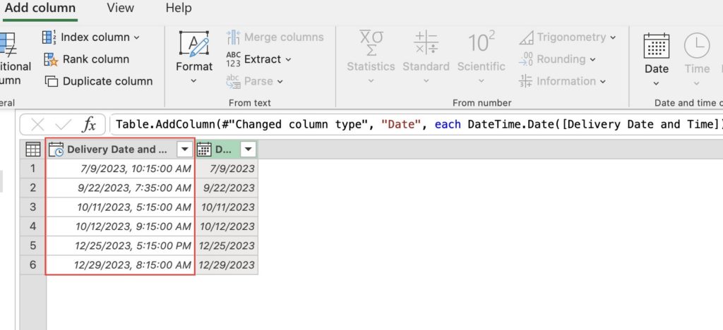
Go to the Add Column tab. Click on Date, then Date Only.
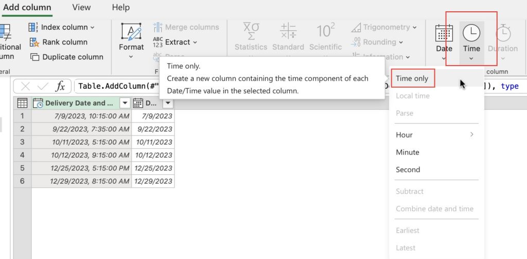
Click back on the Original column and select Time. Click on Time Only.
Click here to learn how Split a Query into Two Parts in Power Query!
Go back to the Home tab.
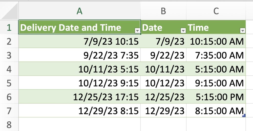
Click the Close & Load button to apply the changes and load the data back into your Excel worksheet.
Conclusion:
There you have it! Separating date and time in Excel is a simple and useful skill when dealing with combined date-time data. Whether you use basic methods like Text to Columns and text functions or advanced techniques involving Power Query, Excel offers a wide range of tools to help you effectively manage your date and time data.
Click here to learn how to use the INT and FIX functions in Excel!
John Michaloudis is a former accountant and finance analyst at General Electric, a Microsoft MVP since 2020, an Amazon #1 bestselling author of 4 Microsoft Excel books and teacher of Microsoft Excel & Office over at his flagship Academy Online Course.
