Show Averages With an Excel Pivot Table

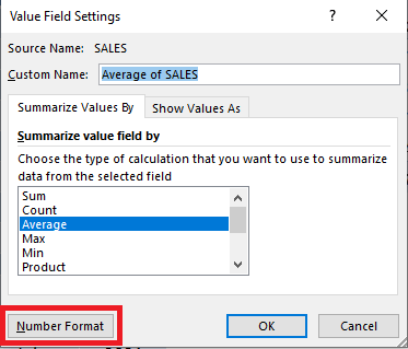
The Summarize Values By option allows you to choose a type of calculation (Sum, Count, Average, Max, Min, Count Numbers Product, StdDev, StdDevp, Var, Varp) to summarize data from the selected field.

As a default when you drop in a values field in the Values area of the Pivot Table it will Sum it for you and give you a Sum of Values.

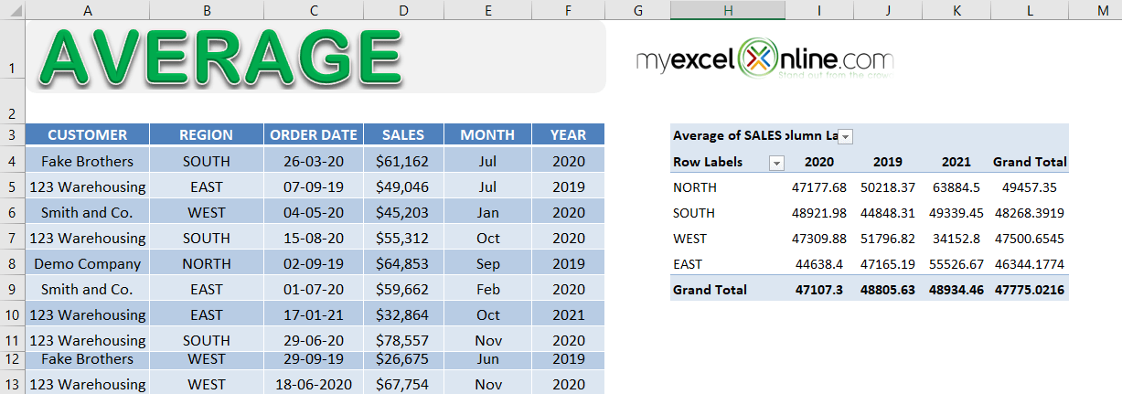
You can change this calculation to an Average very easily, which will show you the Excel pivot table average values for your data.

STEP 1: Click in your data and go to Insert > Pivot Table

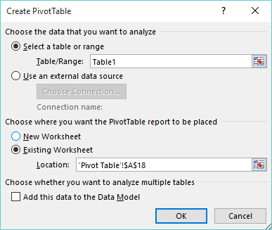
STEP 2: This will bring up the Create Pivot Table dialogue box and it will automatically select your data`s range or table.

In the Choose where you want the PivotTable report to be placed, you can either choose a New Worksheet or an Existing Worksheet.

If you choose a New Worksheet it will place the Pivot Table in a brand new worksheet (e.g. Sheet2).

If you decide to put the Pivot Table in an Existing Worksheet, you will need to select the location by pressing the red arrow, choosing the cell where you want your Pivot Table to be placed, and then pressing the ENTER key twice to confirm.

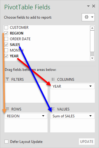
STEP 3: You will now need to drag and drop the Fields in the different areas of your Pivot Table

• Region field in the Row Area
• Year field in Columns Area
• Sales field in Values Area

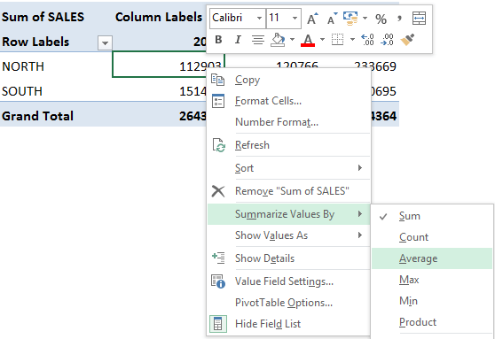
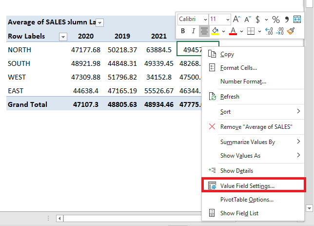
STEP 4:Now that your Pivot Table is set up, you need to Right Click in any of the Pivot Table values and choose Summarize Values By > Average

OR,

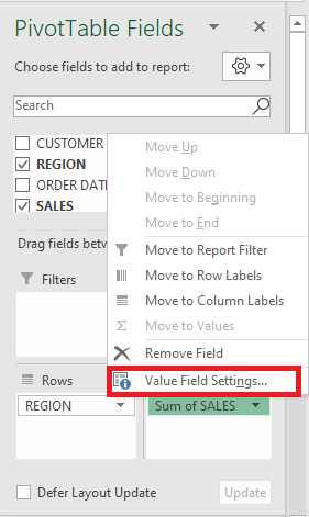
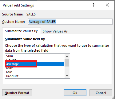
You can simply click on the arrow next to the Sum of Sales field mentioned in the Values Area and select Value Field Setting.

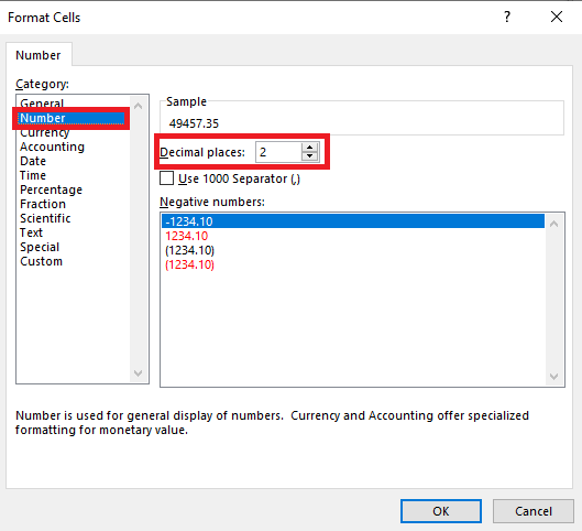
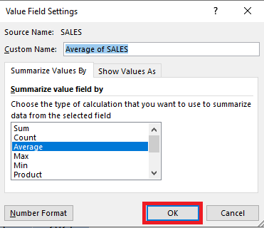
In the Value Field Setting dialog box, Select Average in the Summarize value by and Click OK.

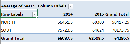
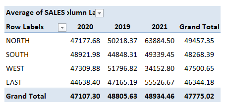
STEP 5: Now you have your Pivot Table report showing the Average Sales values per Region for each year: