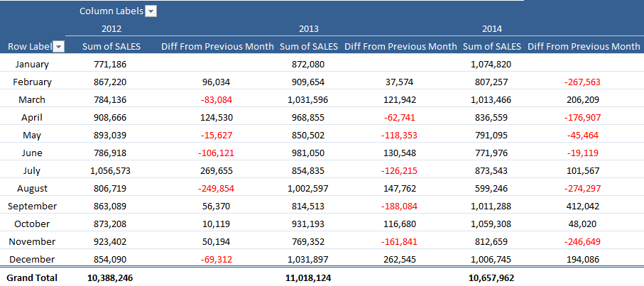
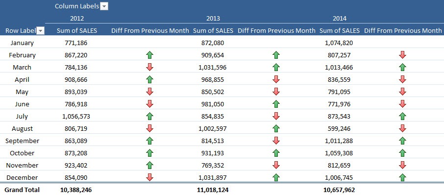
Using a Pivot Table you can show the variance from your previous month’s sales very easily…
See how to Show The Difference From Previous Months With Excel Pivot Tables here
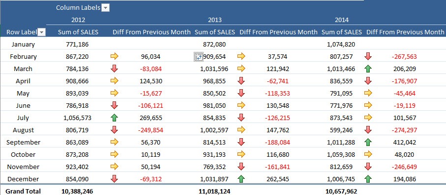
Now that we have the Pivot Table report above, we can show the variances per month using an up/down or directional icon suing Conditional Formatting.
STEP 1: Click on any variance value in the Pivot Table and go to Home > Conditional Formatting > Icon Sets > Directional
STEP 2: This will bring up the Apply Formatting Rule to dialogue box. Choose the 3rd option as this will apply the conditional format on all the values except the Subtotals
Your Pivot Table will look like this:
STEP 3: Now we need to make some edits in the Conditional Formatting Rule in order to get the Icons right.
Go to Home > Conditional Formatting > Manage Rules > Edit Rule
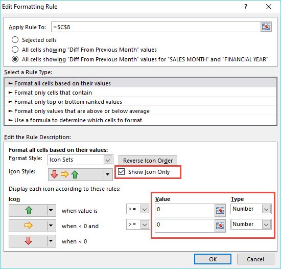
STEP 4: Inside the Edit Formatting Rule box you need to make the following changes:
Value = 0
Type = Number
“Check” the Show Icon Only box and press OK to confirm the changes:
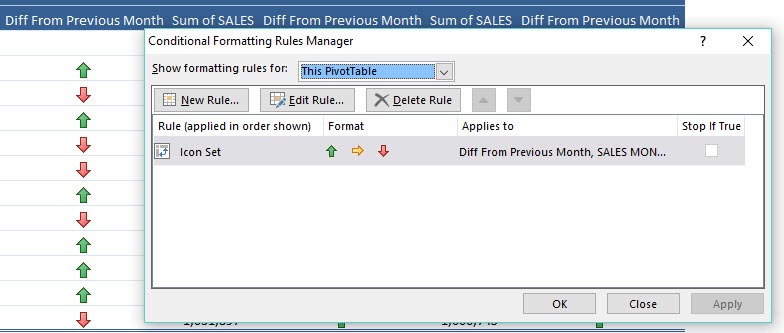
STEP 5: In the next screen you will get the Conditional Formatting Rules Manager. Hit Apply to see the changes and OK to confirm them:
Now you have your Pivot Table showing the differences from the previous months with directional icons only!!!
John Michaloudis is a former accountant and finance analyst at General Electric, a Microsoft MVP since 2020, an Amazon #1 bestselling author of 4 Microsoft Excel books and teacher of Microsoft Excel & Office over at his flagship Academy Online Course.
