Show The Difference From Previous Years With Excel Pivot Tables

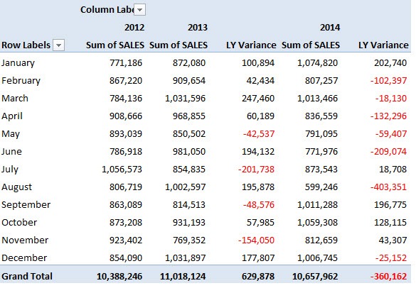
Excel Pivot Tables have heaps of calculations under the SHOW VALUES AS option and one that gets the most use is the Calculate Difference between Two Pivot Tables option.

You can show the values as the Difference From previous months, years, day, etc.  This is just great when your boss asks you how you are tracking to the previous months, years, days.

In this tutorial you will learn how to show:

Let’s look at both of these methods one-by-one!

 

Calculate Difference Between Two Columns

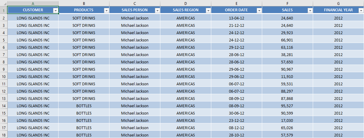
You can use the Pivot Table difference between columns function to calculate Year on Year variance in absolute values. Below is the data that you will be using:

 

Follow the step-by-step tutorial on How to Calculate Difference between Two Pivot Tables and download this Excel workbook to practice along:

 

STEP 1: Insert a Pivot Table by clicking on your data and going to Insert > Pivot Table 

 

STEP 2:In the Create PivotTable dialog box, Select Table range and then click on New Worksheet. Click OK.

 

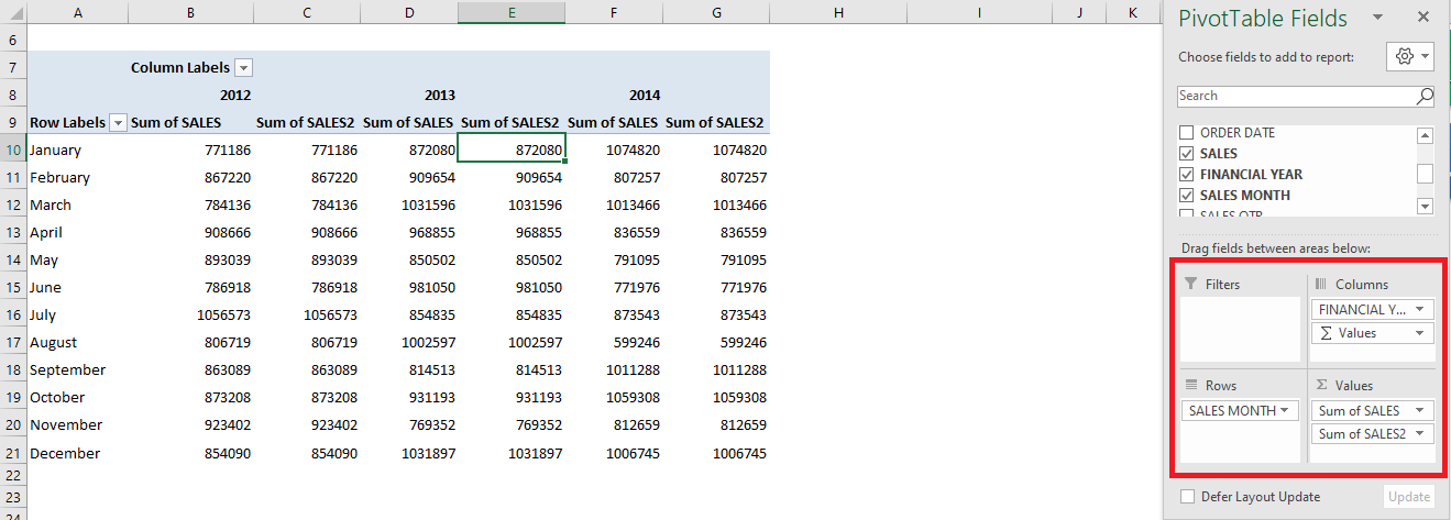
STEP 3: In the ROWS you have to put the Months field, in the COLUMNS the Years field and in the VALUES area the Sales field twice, I explain why below:

 

STEP 4: Now click on the second Sales field’s (Sum of SALES2) drop down and choose Value Field Settings

 

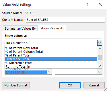
STEP 5: Now you need to select the Show Values As tab and from the drop-down choose the Difference From

 

STEP 6: You need to select the Base Item: (previous) and Base Field: Financial Year and press OK.  So it will read the “Difference from the previous Financial Year”

 

STEP 7: To format the values you need to select the Pivot Table and go to Pivot Table Tools > Analyze/Options > Select > Entire Pivot Table

Then you need to once again go to Pivot Table Tools > Analyze/Options > Select but this time select the Values

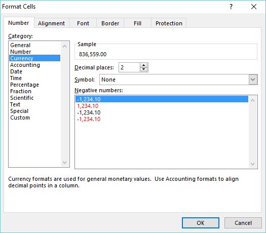
Now press CTRL+1 to bring up the Format Cells dialogue box and make your formatting changes within here and press OK.  

NB: This will fix the number format permanently and any new field that get added into the Pivot Table will have this format.

 

STEP 8: To change the Sum of SALES2 name within the Pivot Table, you need to click on a cell in the Pivot Table that contains Sum of SALES2 and manually make the change, and press Enter

 

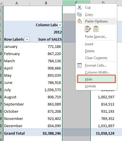
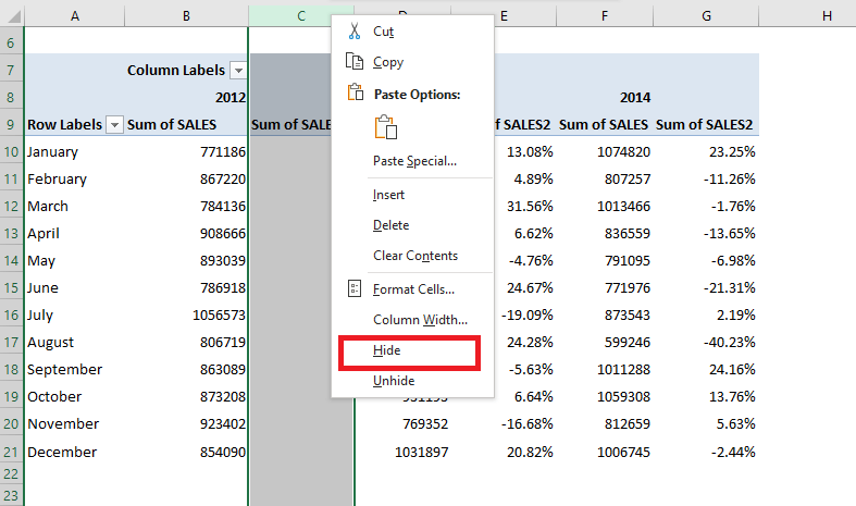
STEP 9: You need to select the whole column that contains the empty values and Right Click and select Hide

 

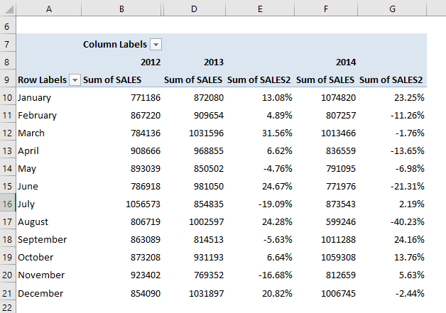
You now have your Pivot Table, all formatted and showing the Difference from the previous Year:

This will provide you with a Pivot Table year over year comparison in absolute terms!

 

Calculate % Difference Between Two Columns

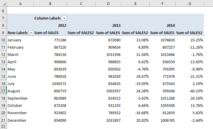
You can also show values as % Difference From. This will display the variance between two years in form of percentage instead of absolute value!

 

Follow the steps below for pivot table calculated field difference between two columns:

STEP 1: Insert a Pivot Table by clicking on your data and going to Insert > Pivot Table 

 

STEP 2:In the Create PivotTable dialog box, Select Table range and then click on New Worksheet. Click OK.

 

STEP 3: Drag and down the following fields in the PivotTable Field dialog box:

• Sales Month in Rows Area
• Financial Year in Columns Area
• Sales in Values Area (Twice)

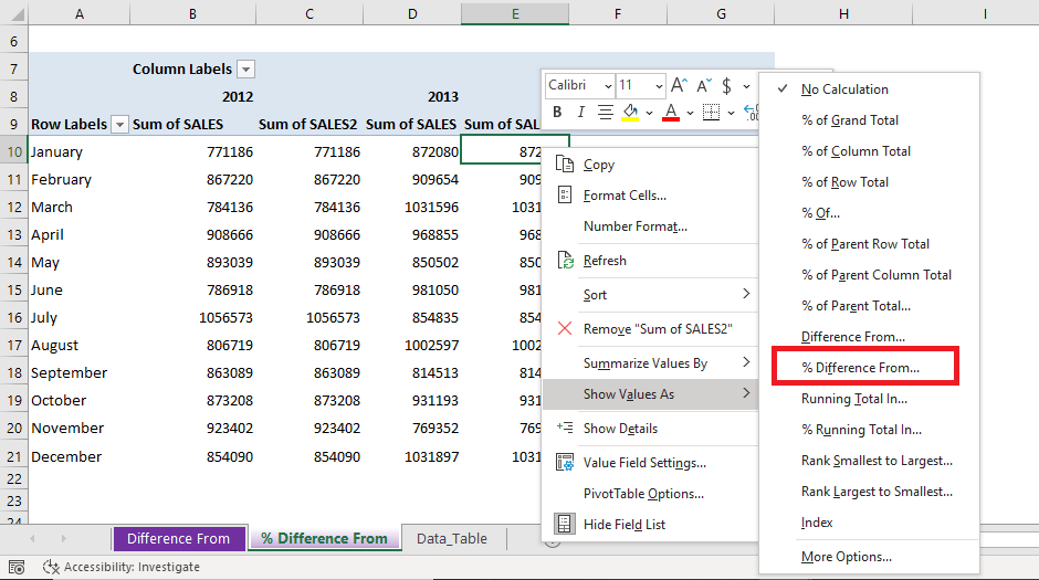
STEP 4: Right Click on the Sum of Sales2 column and select Show Value As > % Difference From.

STEP 5: In the Show Value As dialog box, Select Financial Year as Base Field and (previous) as Base Item. Click OK.

Sum of Sales2 will now display the difference in sales between 2 years in percentage!

STEP 6: Hide the blank Column C. Select Column C > Right Click and Select Hide.

 

And Voila! Your Pivot Table difference between two columns is now ready!

Further Learning:

• Select & Format Fields in Excel Pivot Tables
• Index in Excel Pivot Tables
• Std Dev in Excel Pivot Tables

 

Make sure to download our FREE PDF on the 333 Excel keyboard Shortcuts here: