Show Field and Value Settings in Excel Pivot Tables

With Excel Pivot Tables you can do a lot of stuff with your data! But did you know that you can edit your Field and Value Settings in Pivot Table in multiple places?

Let me show you the different shortcuts so that you can tinker with your Pivot Table!

Download excel workbookField-Value-Field-Settings.xlsx

STEP 1: Let us have a look at the existing Pivot Table. To view the Field Settings, we can do the following:

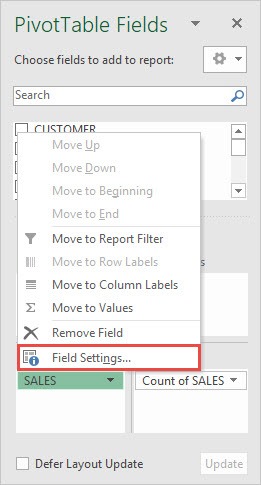
Under PivotTable Fields > Rows > Field Settings

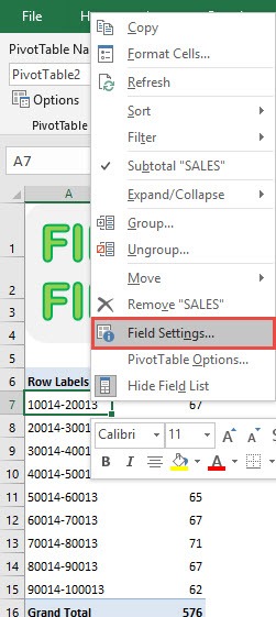
You can also right click on a Row Label and select Field Settings.

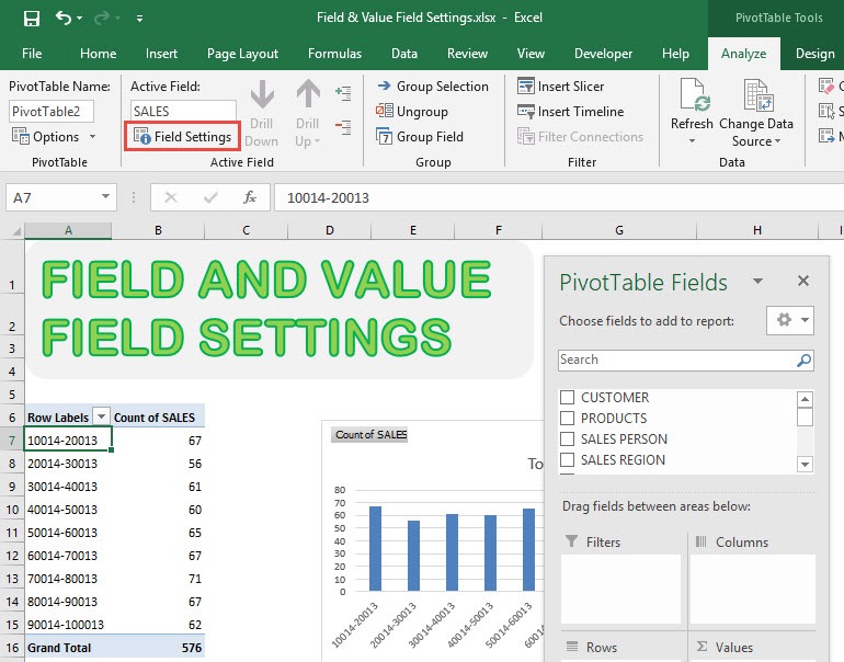
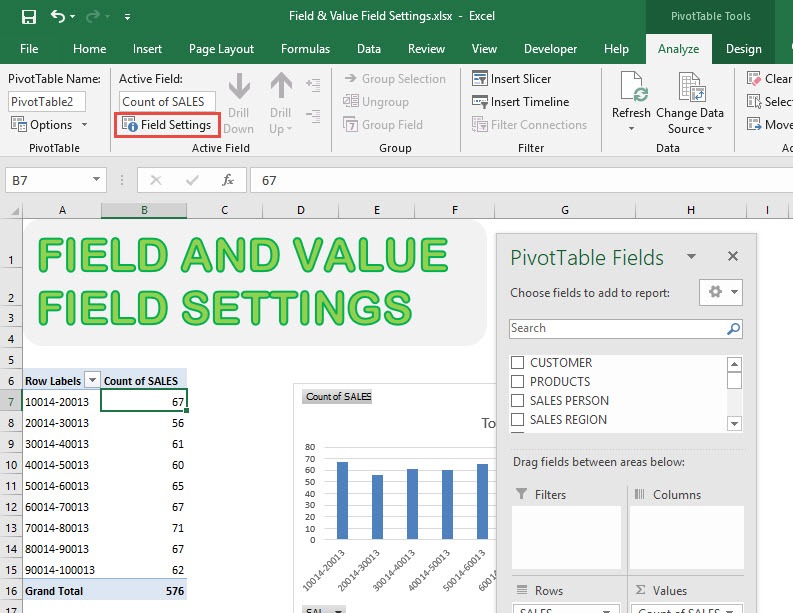
Or while having a row label selected, you can go to PivotTable Tools > Analyze > Active Field > Field Settings

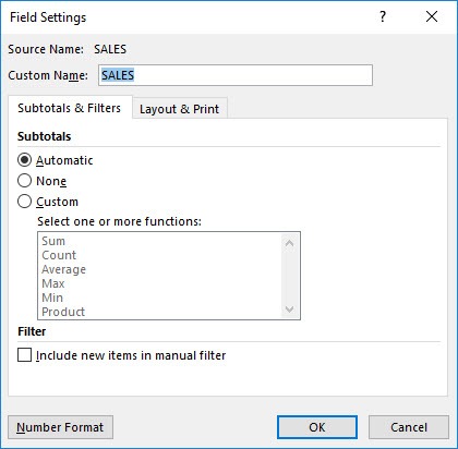
And now you have your Field Settings open!

STEP 2: Now let us see how to access the Value Field Settings.

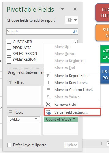
Go to PivotTable Fields > Values> Value Field Settings

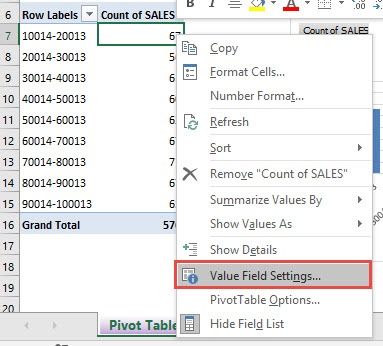
You can also right click on a Value and select Value Field Settings.

Or while having a value selected, you can go to PivotTable Tools > Analyze > Active Field > Field Settings

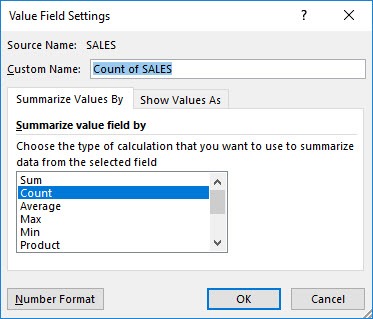
You now have your Value Field Settings!

How to Show Field and Value Field Settings In Pivot Tables

Bryan

Bryan is a best-selling book author of the 101 Excel Series paperback books.