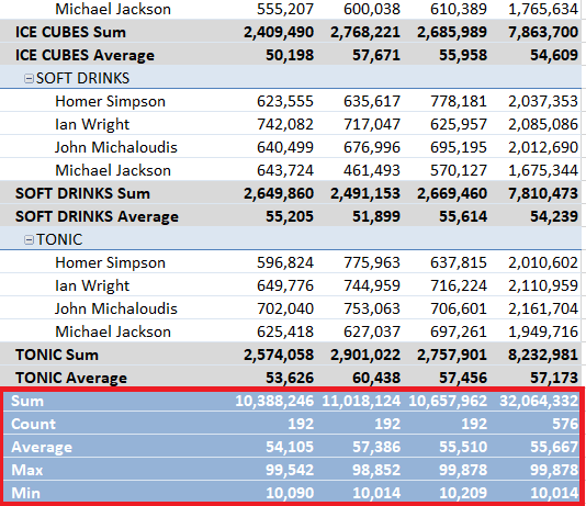
And on top of that, I can customize what value to show. Read on to see how!
Exercise Workbook:
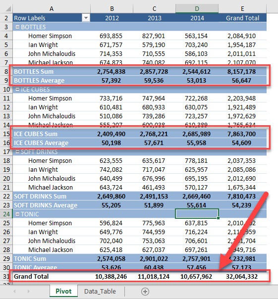
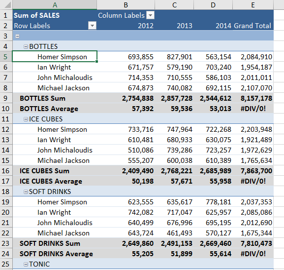
STEP 1: Here is our Pivot Table with multiple Subtotals. However, notice that we only have one Grand Total row.
To know how to insert subtotals in Pivot Table, Click Here.
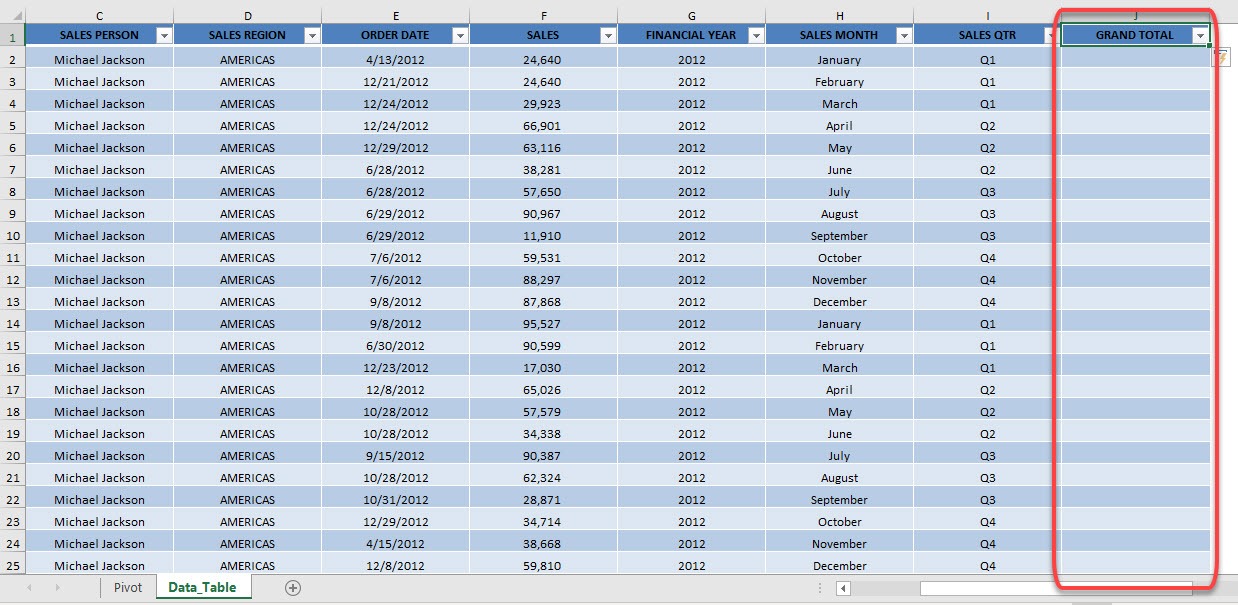
STEP 2: Go to our data source and add a blank column GRAND TOTAL:
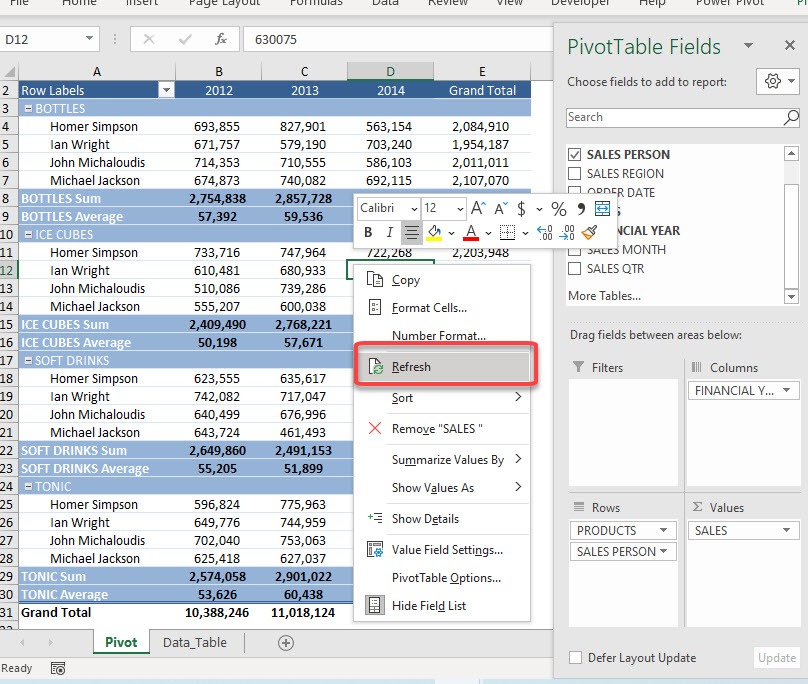
STEP 3: Now right-click anywhere on your Pivot Table and select Refresh
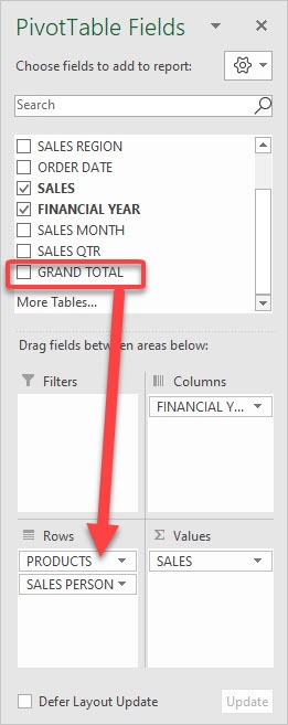
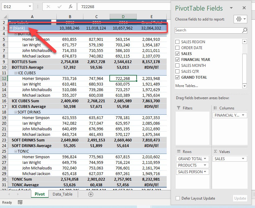
Now the new Grand Total column is now shown there. Drag this to ROWS
You will see our new row being added here.
STEP 4: Press the spacebar and then click on any other cell in the Pivot Table.
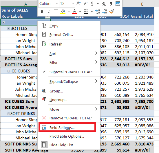
STEP 5: Now let’s do our magic! Right-click on that new row and select Field Settings
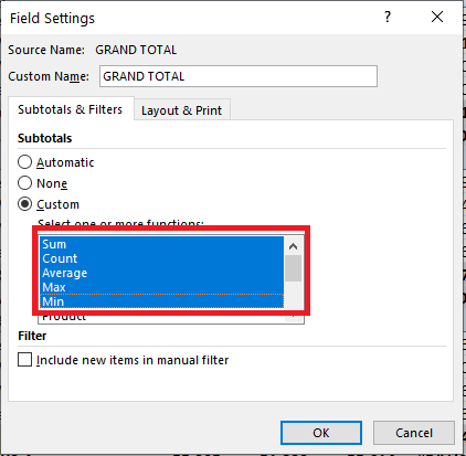
Select Custom and pick the functions that you want to display. Click OK.
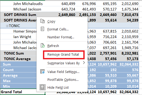
STEP 6: We do not need our Grand Total row anymore. Right-click on it and select Remove Grand Total
Now you have your multiple Grand Totals!
As you can see, there is no direct way to insert multiple grand totals in Pivot. But you can follow the above mentioned steps and easily insert them in your report.
Click here to learn all about Pivot Tables.
Make sure to download our FREE PDF on the 333 Excel keyboard Shortcuts here:
Bryan
Bryan is a best-selling book author of the 101 Excel Series paperback books.
