I am sure that your boss has asked you to come up with a Year on Year variance report at some stage. There are a couple of ways to get him/her an answer.
One is using Formulas, but that will take time to set up and you are exposed to errors!
The other method is the Pivot Table way, which is quick and reduces the risks of making any errors….ah yeah I almost forgot, it is also easy to add new data to your variance analysis!
In the example below I show you how to get the Percentage Difference from Previous Years Values:
STEP 1: Insert a new Pivot table by clicking on your data and going to Insert > Pivot Table > New Worksheet or Existing Worksheet
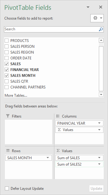
STEP 2: In the ROWS section put in the Sales Month field, in the COLUMNS put in the Financial Year field and in the VALUES area you need to put in the Sales field twice, I explain why below:
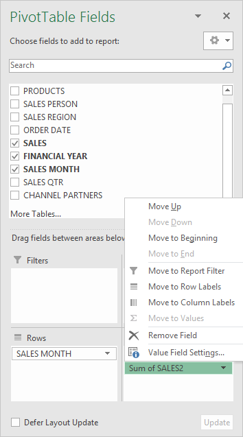
STEP 3: Click the second Sales field’s (Sum of SALES2) drop down and choose Value Field Settings
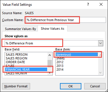
STEP 4: Select the Show Values As tab and from the drop down choose % Difference From. Select Financial Year as the Base Field, and (previous) as the Base Item. This means that we will compute the difference with the previous years in percentage terms.
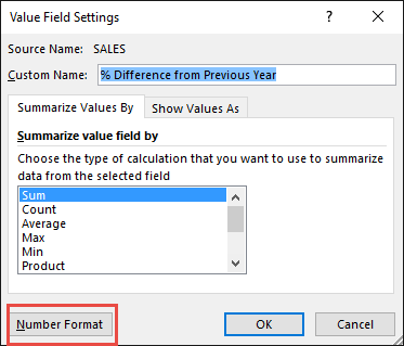
Also change the Custom Name into % Difference from Previous Year to make it more presentable. Click OK.
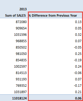
STEP 5: Notice that the % Difference from Previous Year data is in a decimal format that is hard to read:
To format the % Difference from Previous Year column, click the second Sales field’s (% Difference from Previous Year) drop down and choose Value Field Settings.
The goal here is for us to transform numbers from a decimal format (i.e. 0.23), into a percentage format that is more readable (i.e. 23%).
STEP 6: Click the Number Format button.
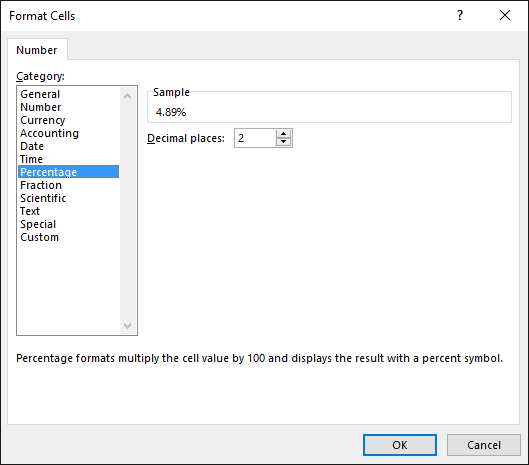
STEP 7: Inside the Format Cells dialog box, make your formatting changes within here and press OK twice.
In this example, we used the Percentage category to make our % Difference from Previous Year numbers become more readable.
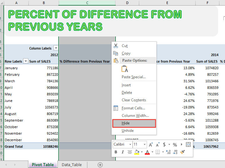
STEP 8: Right click on the columns with the empty columns and click Hide. These columns are empty because there are no previous values it can compare values on. For example the Year 2012 is the first year and has no previous year to compare to.
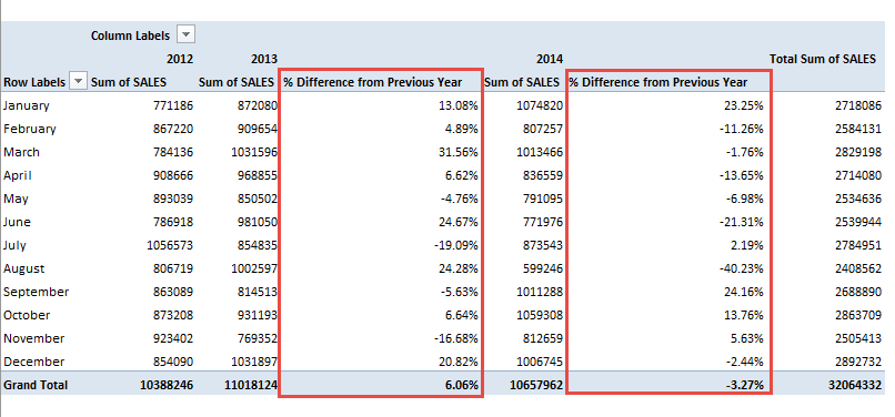
You now have your Pivot Table, showing the % Difference from Previous Year for the sales data of years 2012, 2013, and 2014.
You can see that each red box is the percentage of difference computed against the previous year (i.e. Year 2013 vs Year 2012, and Year 2014 vs Year 2013).
Further Learning:
- Clean Data Set for Pivot Table
- Prepare Data for Excel Pivot Tables
- Move and Remove Fields and Items in Excel Pivot Tables
Bryan
Bryan is a best-selling book author of the 101 Excel Series paperback books.


