Excel Pivot Tables have a lot of useful calculations under the SHOW VALUES AS option and one that can help you a lot is the Excel Pivot Table Percentage of Row Total.
This option will immediately calculate the percentages for you from a table filled with numbers such as sales data, expenses, attendance, or anything that can be quantified.
Want to know How To Show Excel Pivot Table Percentage of Row Total?
*** Watch our video and step by step guide below with a free downloadable Excel workbook to practice ***
Watch on YouTube and give it a thumbs up 👍
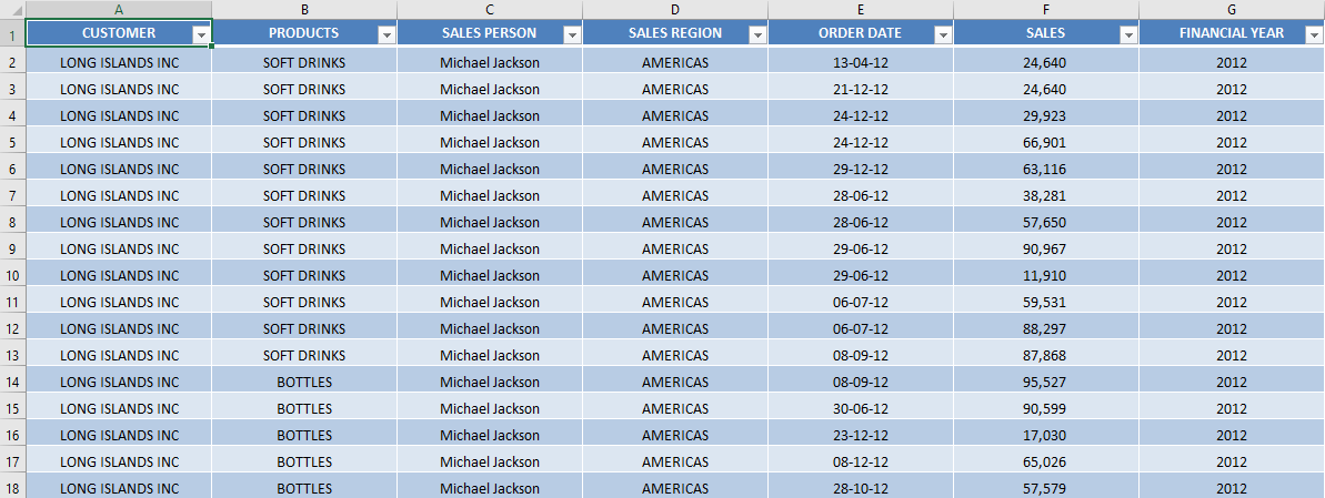
Follow the step-by-step tutorialbelow to understand how to show Excel Pivot Table Percentage of Row Total and make sure to download the workbook to follow along:
STEP 1: Select any cell in the Data Table
STEP 2: Go to Insert > PivotTable.
STEP 3: In the Create PivotTable dialog box, select table range and New Worksheet and then Click OK.
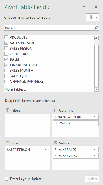
STEP 4: In the ROWS section put in the Sales Person field, in the COLUMNS put in the Financial Year field and in the VALUES area you need to put in the Sales field twice, I explain why below:
A Pivot Table will be created and looks like this:
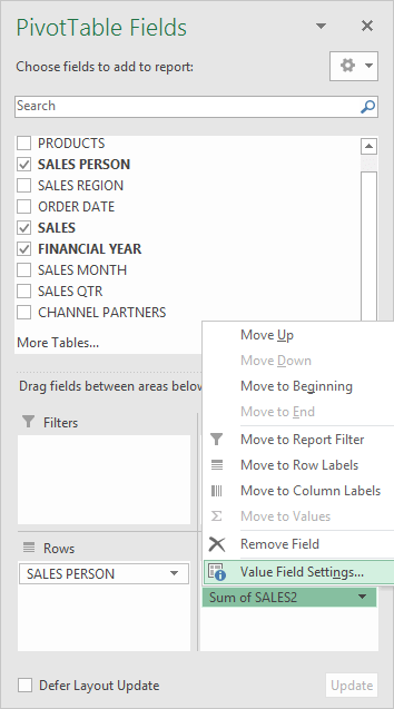
STEP 5:Click the second Sales field’s (Sum of SALES2) drop down and choose Value Field Settings
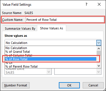
STEP 6: Select the Show Values As tab and from the drop down choose % of Row Total.
Also, change the Custom Name into Percent of Row Total to make it more presentable. Click OK.
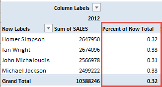
STEP 7: Notice that the Percent of Row Totaldata is in a decimal format that is hard to read:
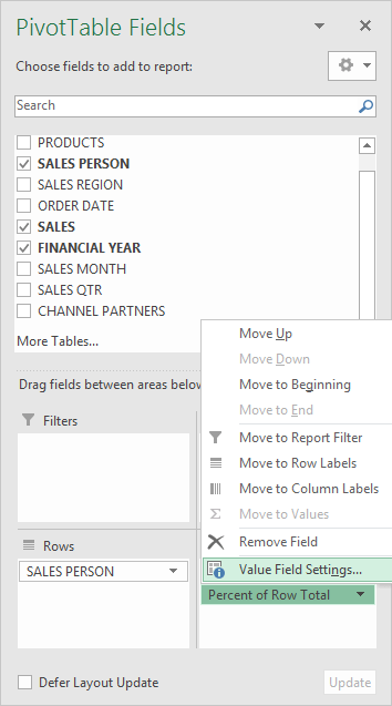
To format the Percent of Row Totalcolumn, click the second Sales field’s (Percent of Row Total) drop down and choose Value Field Settings.
The goal here is for us to transform numbers from a decimal format (i.e. 0.23), into a percentage format that is more readable (i.e. 23%).
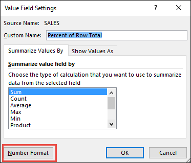
STEP 8: Click the Number Format button.
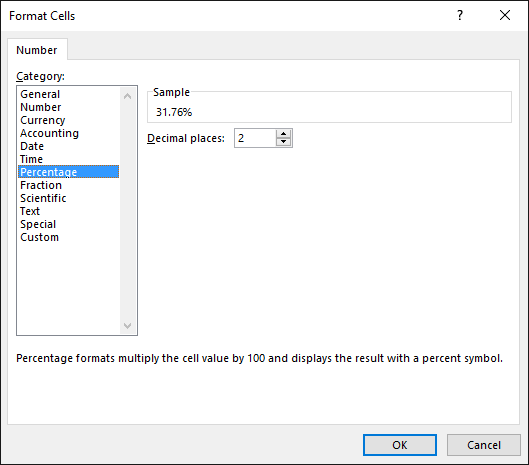
STEP 9: Inside the Format Cells dialog box, make your formatting changes within here and press OK twice.
In this example, we used the Percentage category to make our Percent of Row Total numbers become more readable.
You now have your Pivot Table, showing the Percent of Row Total for the sales data of years 2012, 2013, and 2014.
All of the sales numbers are now represented as a Percentage of each row (Years 2012, 2013 and 2014), which you can see on each row is represented as 100% in totality.
Particularly the yellow highlighted ones would total to 100% for the first row:
Further Learning:
- Show The Difference From Previous Months With Excel Pivot Tables
- Show The Percent of Row Total With Excel Pivot Tables
- Show The Percent of Difference From Previous Years With Excel Pivot Tables
Make sure to download our FREE PDF on the 333 Excel keyboard Shortcuts here:
You can learn more about how to use Excel by viewing our FREE Excel webinar training on Formulas, Pivot Tables, Power Query, and Macros & VBA!
Bryan
Bryan is a best-selling book author of the 101 Excel Series paperback books.

