You have your Pivot Table ready, all sorted nicely both from a row and column perspective. However you just need that one minor sorting tweak or two.
Well, Excel seemingly has a lot of tricks and you can even sort an Excel Pivot Table manually!
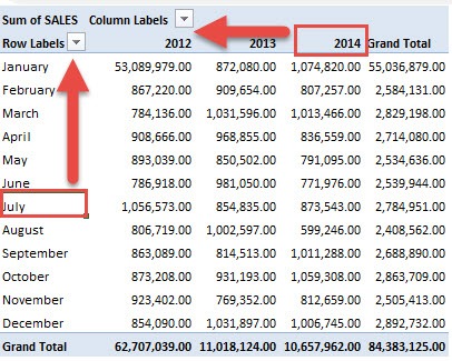
For our example, let’s see this Pivot Table below. It is sorted by years (2012-2014), and months (Jan-Dec).
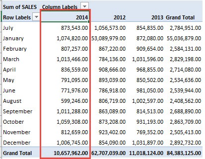
But what if we want to move July to the top, and the year 2014 as the first column year?
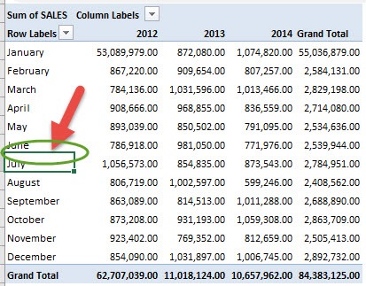
STEP 1: To manually sort a row, click on the cell you want to move. Hover over the border of that cell until you see the four arrows:
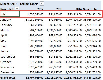
Left mouse click, hold and drag it to the position you want (i.e. upwards to the first row)
We dragged it to the top so it’s now the first row!
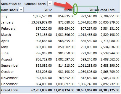
STEP 2: To manually sort a column, click on the cell you want to move. Hover over the border of that cell until you see the four arrows.
Left mouse click, hold and drag it to the position you want (i.e. all the way to the left)
Voila! You have successfully manually sorted your Pivot Table!
EXTRA TIP: You can click inside a cell e.g. January, and start typing in another month, like August. This will also manually sort your Pivot Table items.
Further Learning:
- Sort Largest to Smallest Grand Totals With Excel Pivot Tables
- SORT Formula in Excel
- SORTBY Formula in Excel
Bryan
Bryan is a best-selling book author of the 101 Excel Series paperback books.
