I knew that I could sort virtually anywhere with Excel Pivot Tables, but I was surprised that I could even Excel Pivot Table Sort by Grand Total!
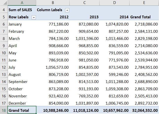
Below I have an Excel Pivot Table that consists of Sales Numbers over a three-year period.
Want to know How To Show Excel Pivot Table Sort by Grand Total?
Watch Sort Pivot Table by Grand Total on YouTube and give it a thumbs-up!

Follow the step-by-step tutorial on Excel Pivot Table Sort by Grand Total and download this Excel workbook to practice along:
download excel workbookSort-Largest-to-Smallest-Grand-Totals.xlsx
In the example below I show you how to Sort by Largest to Smallest based on Grand Totals.
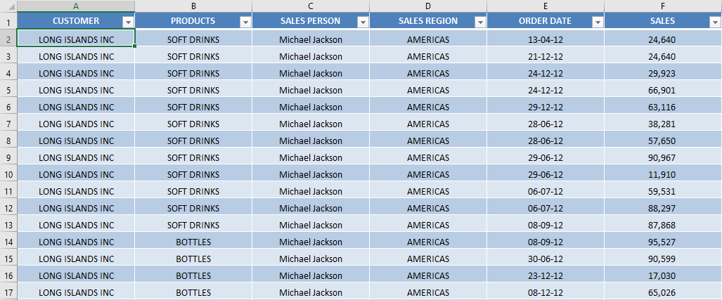
STEP 1: Select any cell in the data table.
STEP 3: Insert a new Pivot In the Create PivotTable dialog box, select the table range and New Worksheet, and then click OK.
STEP 4: In the ROWS section put in the Sales Month field, in the COLUMNS put in the Financial Year field and in the VALUES area you need to put in the Sales field:
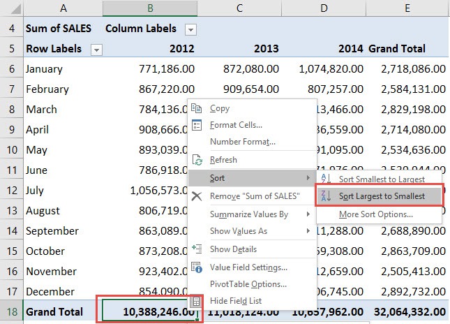
STEP 5: Right-click on a Grand Total below at the bottom of the Pivot Table. Go to Sort > Sort Largest to Smallest
(If you cannot see the Grand Totals, click in your Pivot Table and go to the ribbon menu and select PivotTable Tools > Design > Grand Totals > On for Rows and Columns)
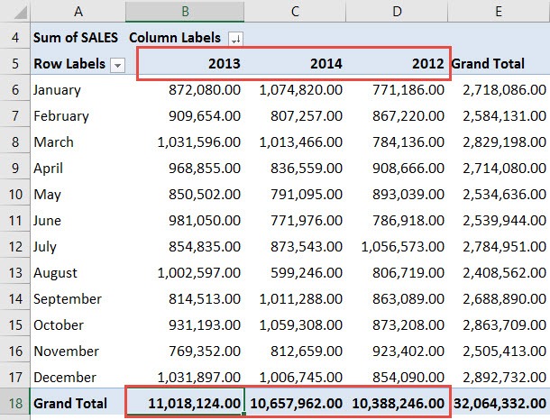
STEP 6: This will sort our grand totals by descending order.
See that our years are now arranged in this order: 2013, 2014, 2012.
This completes our tutorial on How to Sort Grand Total in Pivot Table!
Further Learning:
- Sort All Worksheets By Name Using Macros In Excel
- SORT Formula in Excel
- Sort an Excel Pivot Table Manually
Make sure to download our FREE PDF on the 333 Excel keyboard Shortcuts here:
Bryan
Bryan is a best-selling book author of the 101 Excel Series paperback books.


