Split the Date Using Power Query or Get & Transform

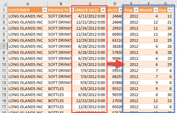
Power Query or Get & Transform (In Excel 2016) lets you perform a series of steps to transform your Excel data.  One of the steps it allows you to take is to split your date into year, month and day for easier processing.

Download excel workbookSplit-the-Date.xlsx

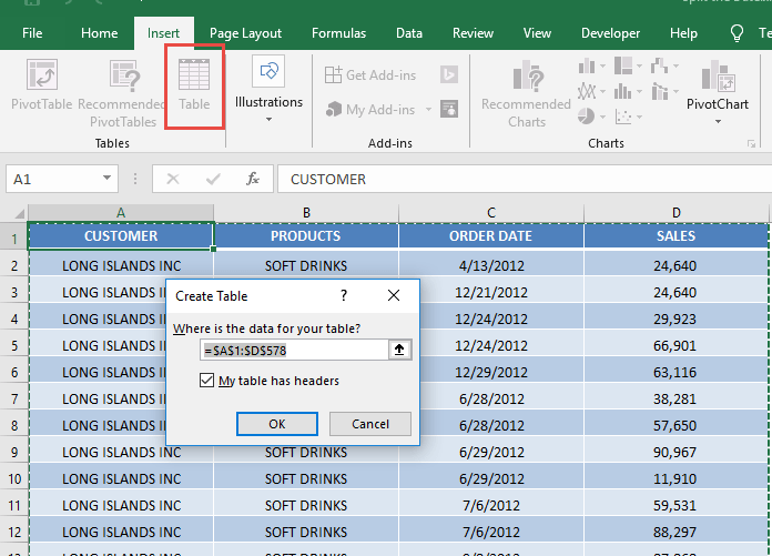
STEP 1: Select your data and turn it into an Excel Table by pressing the shortcut Ctrl + T or by going to Insert > Table

STEP 2: Go to Data > Get & Transform > From Table (Excel 2016) or Power Query > Excel Data > From Table (Excel 2013 & 2010)

Excel 2016:

Excel 2013 & 2010:

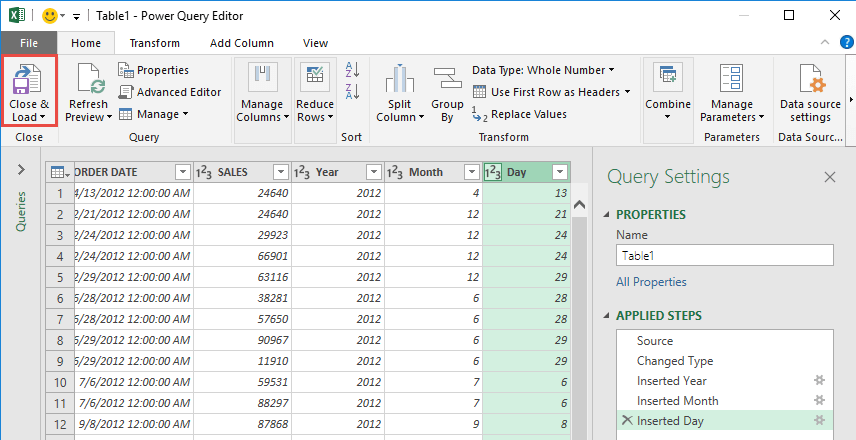
STEP 3: This will open up the Power Query Editor. Let us now get the Year, Month and Day.

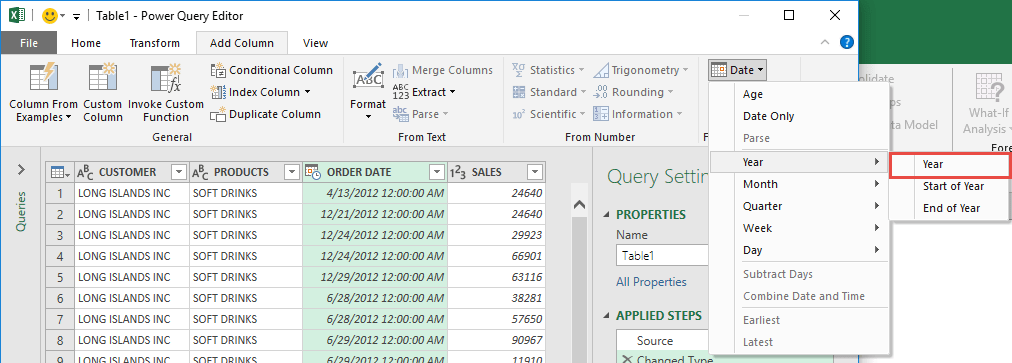
Make sure the Order Date column is selected. Go to Add Column > From Date & Time > Date > Year> Year

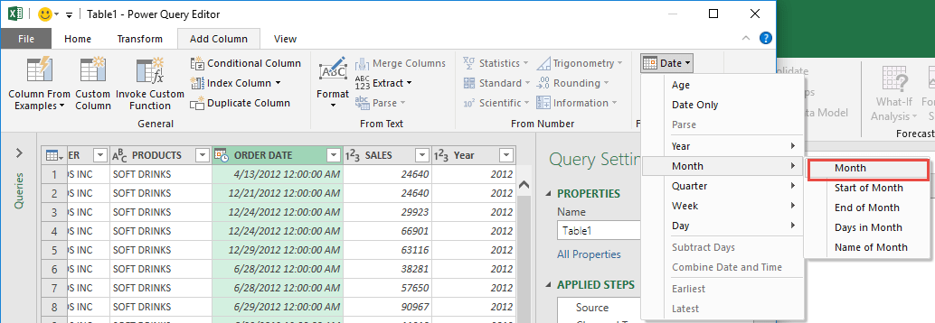
Make sure the Order Date column is selected. Go to Add Column > From Date & Time > Date > Month > Month

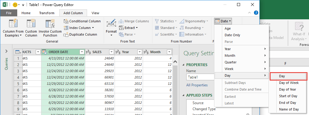
Make sure the Order Date column is selected. Go to Add Column > From Date & Time > Date > Day > Day

STEP 4: Click Close & Load from the Home tab and this will open up a brand new worksheet in your Excel workbook with the updated records!

You now have your dates split to Year, Month and Day!

How to Split the Date in Excel Using Power Query

Bryan

Bryan is a best-selling book author of the 101 Excel Series paperback books.