Std Dev in Excel Pivot Tables

Let us explore how to get the std dev in Pivot Table, this shows the amount by which members of a group are different from the average value for the group.

Exercise Workbook:

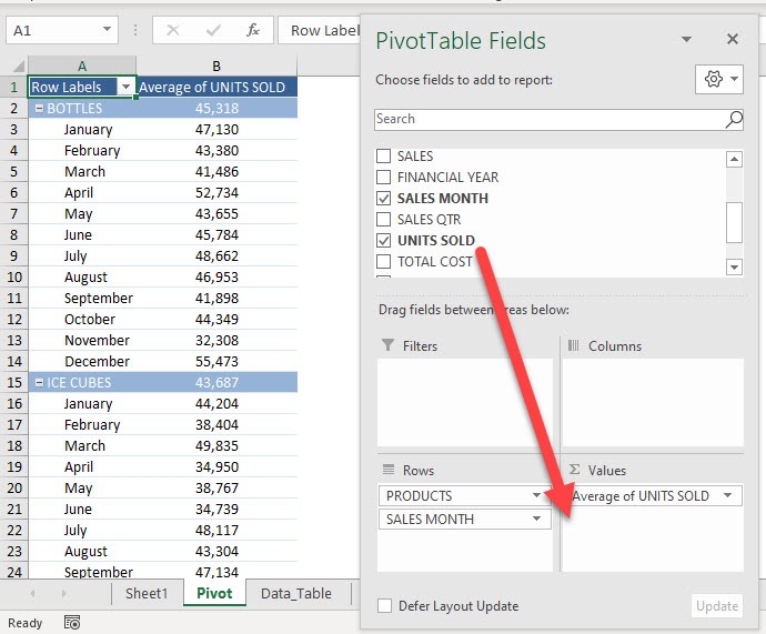
STEP 1: Here is our Pivot Table. Drag UNITS SOLD to the Values Area

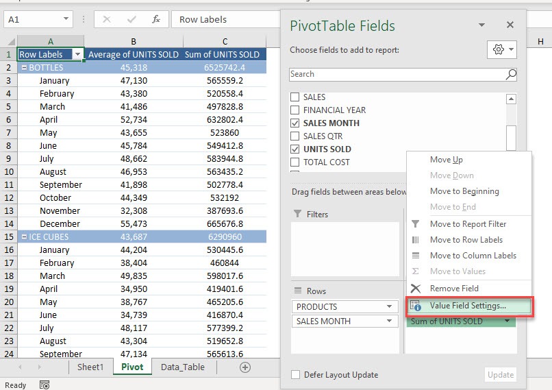
STEP 2: This will default to Sum of UNITS SOLD. Let us change that by clicking on the arrow and selecting Value Field Settings

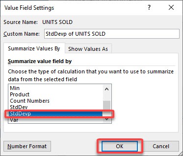
STEP 3: Select StdDevp and click OK.

We will use the StdDevp function as we have the complete data (population) used in the calculation. When only a portion of the data is used, then StdDev should be used instead.

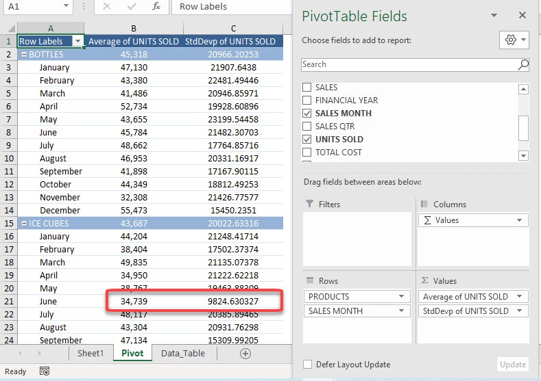
Now you have your Standard Deviation! You can see for ICE CUBES on the month of June the Standard Deviation is quite low. This means that the values on the units sold for that month is fairly close to the average of 34,739.

Did you know that the square of the standard deviation will give you the variance value? Click here to know more!

Make sure to download our FREE PDF on the 333 Excel keyboard Shortcuts here:

Bryan

Bryan is a best-selling book author of the 101 Excel Series paperback books.

See also  Filter by Labels - Numerical Text