How to Apply Strikethrough in Excel – 3 Easy Methods

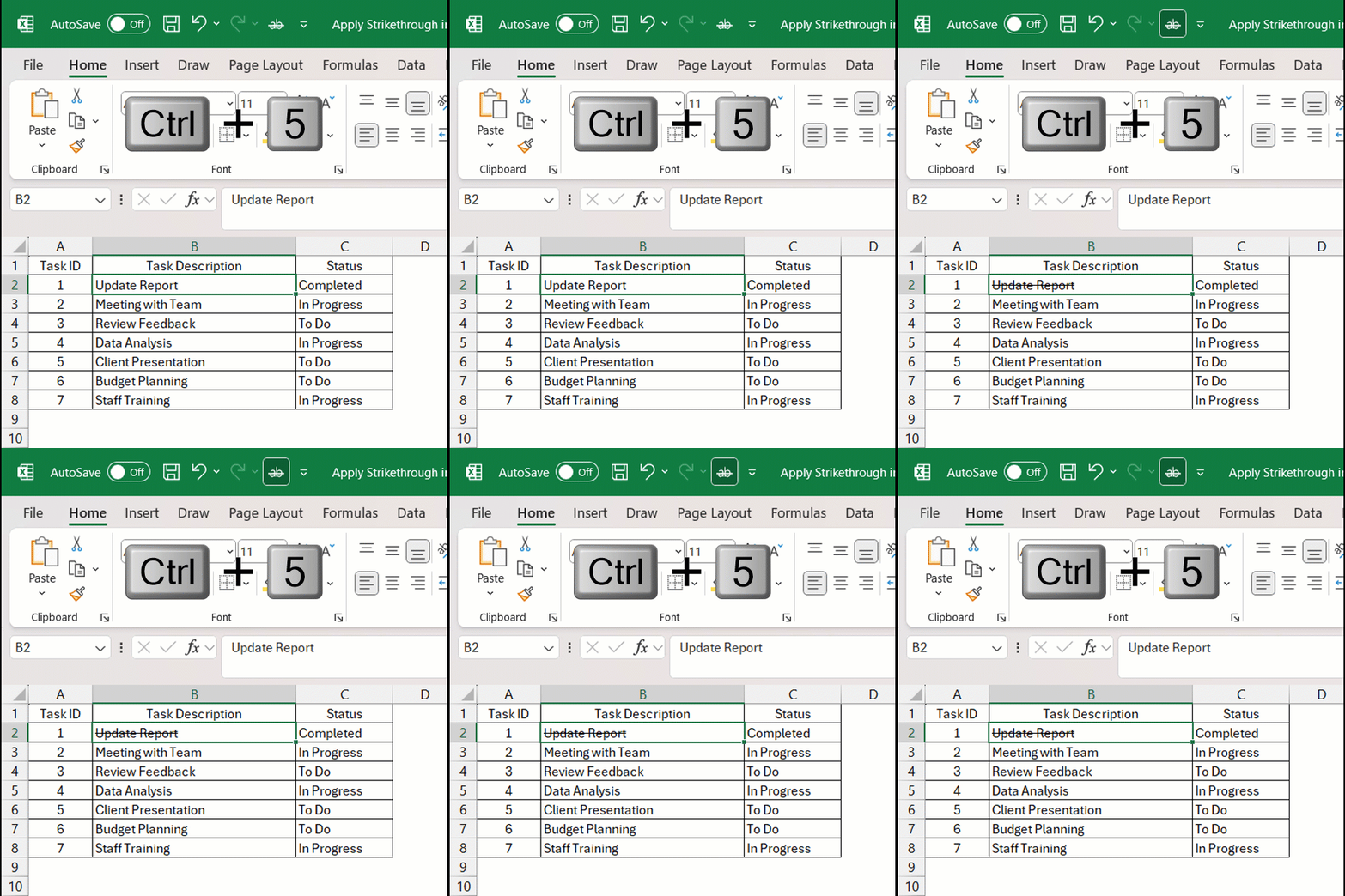
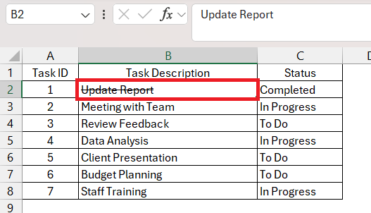
Strikethrough is a formatting technique that adds a horizontal line through the middle of the text. It can be used to indicate to users that the information has been revised, is not valid anymore, or has been completed. It helps users easily identify changes or updates in the spreadsheet while still showing the old information.

In this article, we will cover 3 different methods to apply strikethrough in Excel –

Let’s look at each of these methods in detail.

 

Download the Excel Workbook below to follow along and understand how to Apply Strikethrough in Excel –

download excel workbookApply-Strikethrough-in-Excel.xlsx

 

Method 1 – Using Keyboard Shortcut

The quickest way to apply strikethrough in Excel is through a simple keyboard shortcut. You can easily apply strikethrough using the shortcut – Ctrl + 5. Once you press Ctrl + 5, the formatting will automatically be applied to the entire contents of the cell.

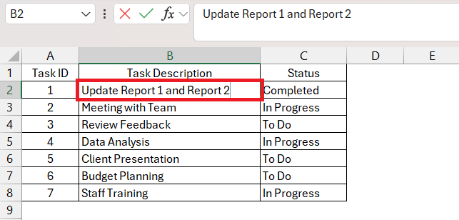
You can also select a single cell, a range of cells, or even an entire column or row and follow the same step to apply strikethrough. In some cases, you may want to strike out only a part of the text within the cell. This can also be achieved by following the steps below –

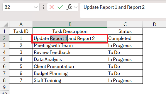
STEP 1: Double-click the cell to enter the edit mode.

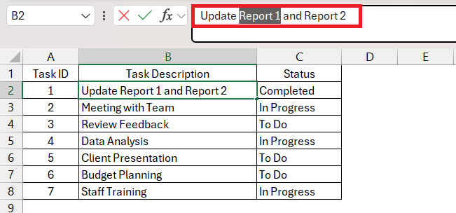
STEP 2: Highlight the part of the text that you want to strike out.

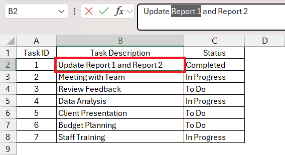
STEP 3: Press Ctrl + 5.

The selected text will be strikethrough.

What if you wish to remove this formatting? Choose the text where you wish to remove the strikethrough, and then use the keyboard shortcut Ctrl + 5.

 

Method 2 – Using Format Cell Option

This method provides more control over formatting options. Follow the steps below to apply strikethrough using the format cell option –

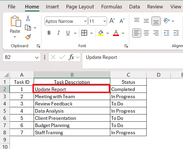
STEP 1: Select the cell where you want to strikethrough.

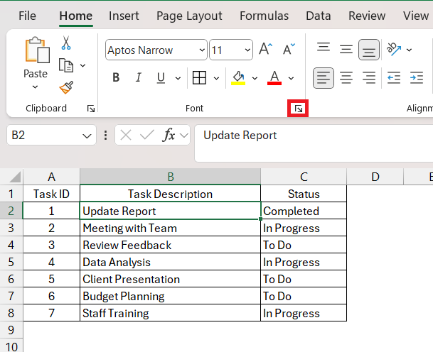
STEP 2: Go to the Home tab and within the font section, click on the Font setting button. This is the small arrow at the bottom right corner of the section.

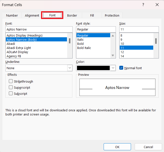
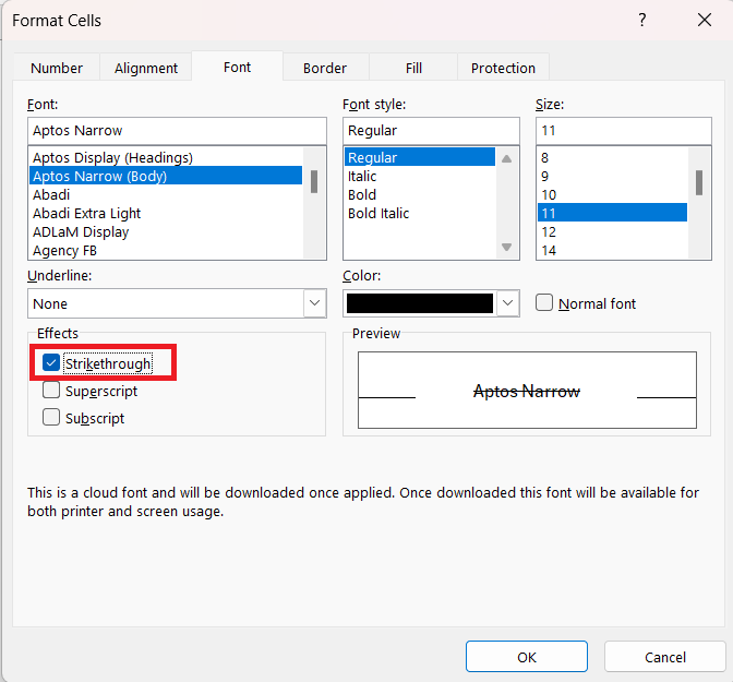
STEP 3: In the Format Cells dialog, go to the Font tab.

STEP 4: Check the Strikethrough option in the Effects section and click OK to apply the formatting.

The strikethrough formatting will be applied to the selected cell.

 

Method 3 – Using Quick Access Toolbar

The Quick Access Toolbar in Excel is a customizable toolbar located at the top of the Excel window, near the Ribbon. It provides users with a convenient and quick way to access frequently used commands and features, regardless of the active tab in the Ribbon.

If you frequently use strikethrough in Excel, you can add it to the Quick Access Toolbar for easy access. Follow these steps below to use QAT to apply strikethrough formatting –

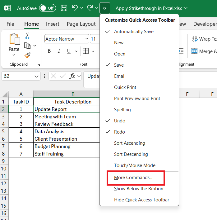
STEP 1: Click on the small arrow next to the Quick Access Toolbar and select More Commands.

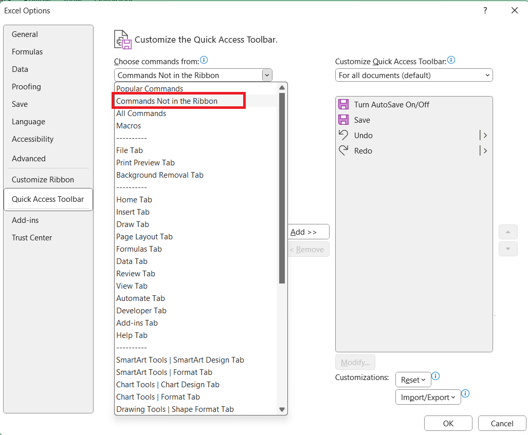
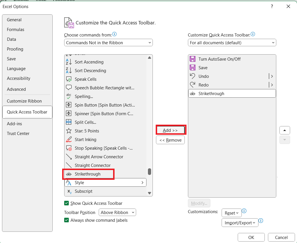
STEP 2: In the Excel Options dialog box, select Commands Not in the Ribbon from the Choose commands from dropdown.

STEP 3: Select Strikethrough from the list on the left and then click Add.

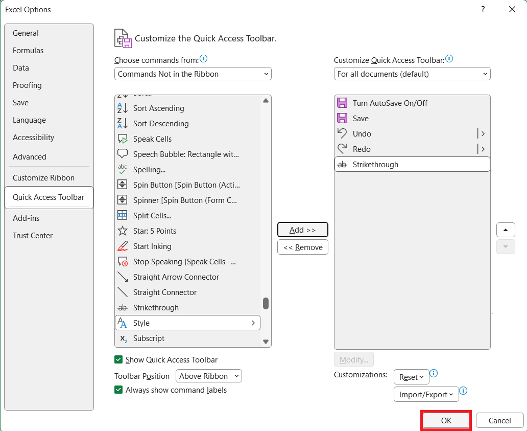
STEP 4: Click OK to close the dialog box.

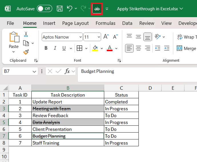
Now, you can simply click on the newly added strikethrough icon in the Quick Access Toolbar to apply the formatting.

 

Conclusion

In conclusion, Strikethrough in Excel helps users improve data presentation and communication. Its ability to signify changes or completion is a valuable tool for users managing spreadsheets. You can either employ the convenient keyboard shortcut, utilize the Format Cells option, or incorporate the Quick Access Toolbar for seamless access.

These three methods offer flexibility and efficiency in applying strikethrough formatting in Excel. Choose the method that best fits your workflow and make your data more visually impactful and communicative.