Sumproduct & Weighted Averages

Sumproduct & Weighted Averages

What does it do?

It returns the sum of the products of corresponding ranges or arrays

Formula breakdown:

=SUMPRODUCT(array1, [array2], [array3]…)

What it means:

=SUMPRODUCT(this array, with that array…)

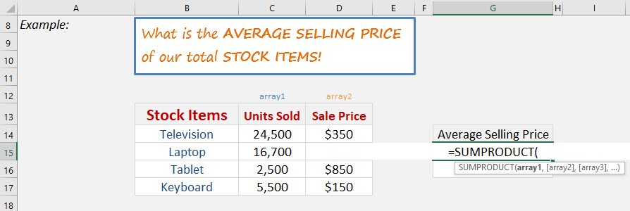
A quick way to calculate the weighted average of two lists of data is to use the SUMPRODUCT formula.  A weighted average can be used to determine the average salary of employees, the average grade of an exam or the average selling price of a company´s stock list, as can been seen below.

We want to get the average selling price of our total stock items. This is easily achievable with the SUMPRODUCT formula! We will use this to calculate the total value of the items, then divide this by the total number of units to get the average selling price.

STEP 1: We need to enter the SUMPRODUCT function in a blank cell:
=SUMPRODUCT(

STEP 2: The SUMPRODUCT arguments:

Array1

What is the first array that contains the data?

We want to get the units sold so select those values.
=SUMPRODUCT(C14:C17,

Array2

What is the second array that contains the data?

We want to get the sale price sold so select those values. The values will be multiplied against the first array that we got.
=SUMPRODUCT(C14:C17, D14:D17)

STEP 3: Now we have the total value, we can easily get the average value by dividing by the total number of items.
=SUMPRODUCT(C14:C17, D14:D17) / SUM(C14:C17)

With just this single formula, we are able to get the average selling price without the need of extra helper columns!

John Michaloudis

Founder & Chief Inspirational Officer

at

MyExcelOnline.com

John Michaloudis is a former accountant and finance analyst at General Electric, a Microsoft MVP since 2020, an Amazon #1 bestselling author of 4 Microsoft Excel books and teacher of Microsoft Excel & Office over at his flagship Academy Online Course.