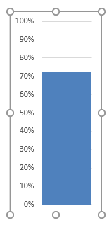
Thermometer Charts are one of the many Charts you can create in Excel. It does not really exist in Excel, however we can get creative and create our own.
A Thermometer Chart gives you a good view of the percentage of progress made on your project, budget etc.
We are going to use a Column Chart and customize it to make it look like a thermometer.
In this example I show you how easy it is to insert a Thermometer Chart using Excel.
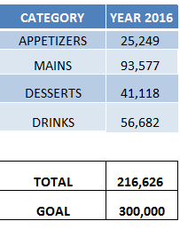
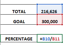
STEP 1: Given your data, ensure that you have the Percentage computed.
We have the Percentage computed as the Total divided by the Goal Amount.
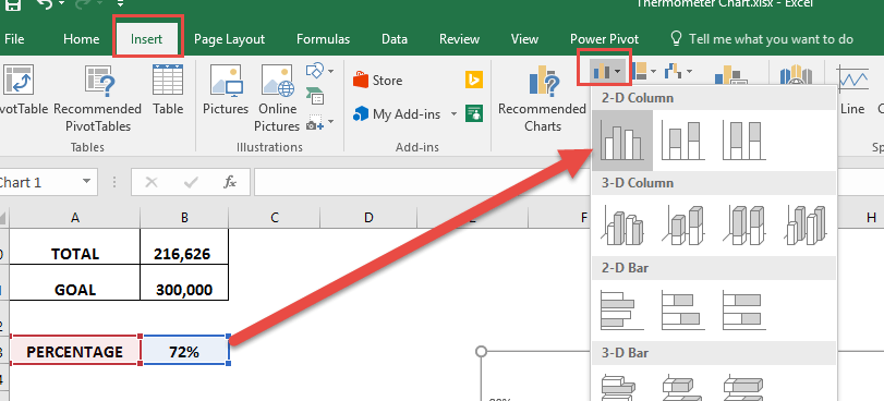
STEP 2: Select the Percentage value, and select Insert > Column Charts > 2-D Clustered Column
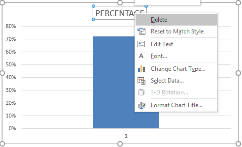
STEP 3: Right-click on the Header and Click Delete.
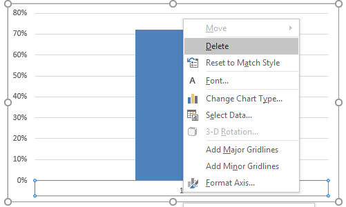
STEP 4: Right-click on the bottom column name and Click Delete
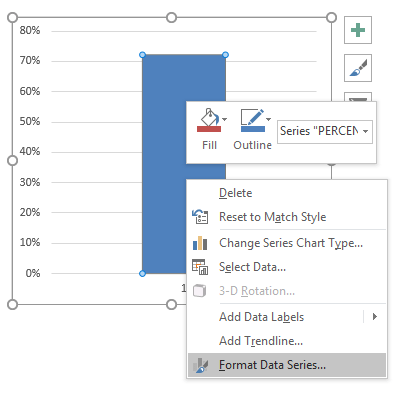
STEP 5: Right click on the Column itself, and Select Format Data Series.
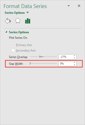
Set the Gap Width to 0%. This will ensure the column fills our entire chart.
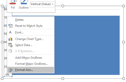
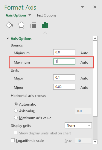
STEP 6: Right click on the Column percentages, and Select Format Axis.
Set the Maximum to 1. This will ensure our range is from 0% to 100%.
STEP 7: Resize the chart to a smaller size. You now have your Thermometer Chart ready.
Update your data values and see the chart go up and down!
Bryan
Bryan is a best-selling book author of the 101 Excel Series paperback books.

