Timeline Slicers In Microsoft Excel

Have a Pivot Table with dates involved? Did you know you can create a cool timeline slicer wherein you can dynamically filter your data based on date ranges?

You will be blown away by what it can do! And with just a couple of clicks!

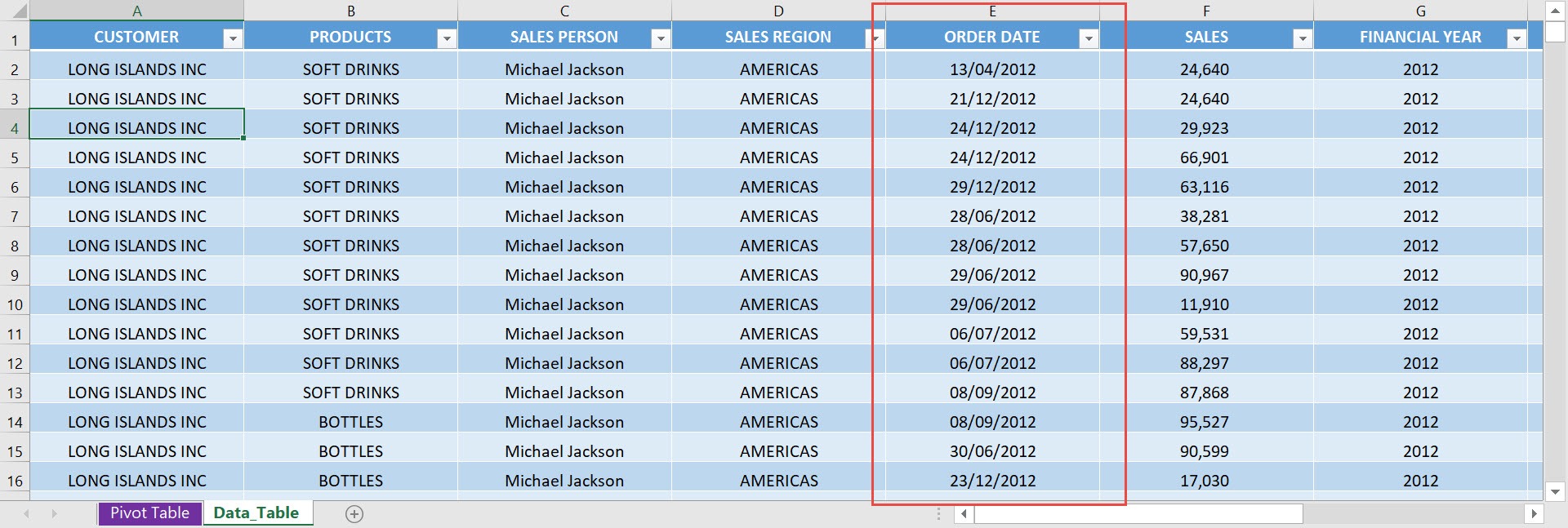
Our data has an Order Date column that we will use for the Slicer.

Download excel workbookTimeline-Slicers.xlsx

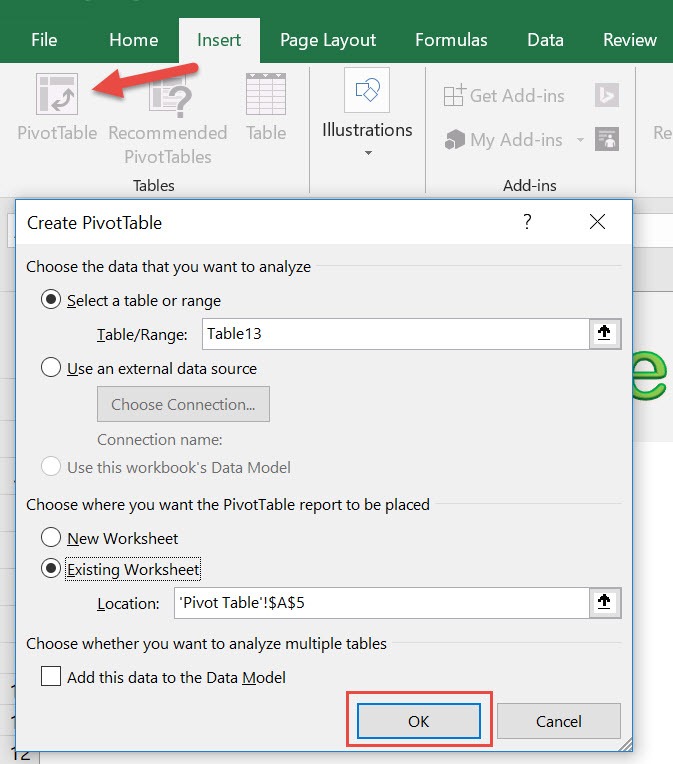
STEP 1: Insert a new Pivot table by clicking on your data and going to Insert > Pivot Table > New Worksheet or Existing Worksheet

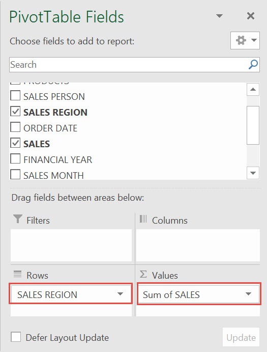
STEP 2: In the ROWS section put in the Sales Region field.  In the VALUES section put in the Sales field.

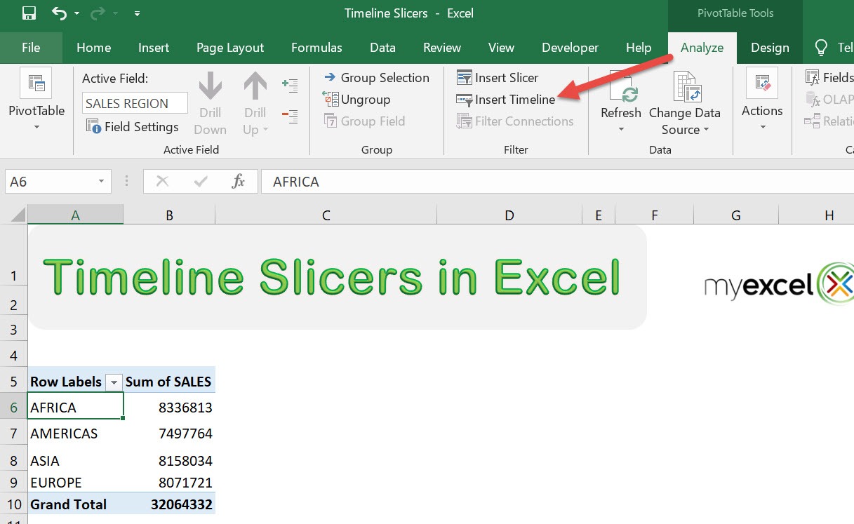
STEP 3: Let us now add our timeline slicer! Go to PivotTable Tools> Analyze > Filter > Insert Timeline

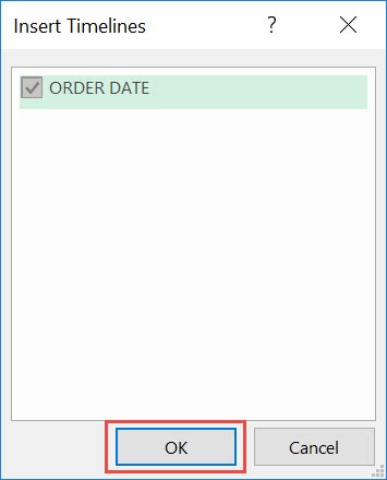
STEP 4: Make sure ORDER DATE is ticked. Click OK.

And now you have your Timeline Slicer! You can play around and set different date ranges, then the pivot table data will also adjust accordingly.

See this example where we tried Jan 2012 – Mar 2012. You can also change the unit (e.g. months, years, etc.) of your slicer!

How to Create a Timeline Slicer in Excel

Bryan

Bryan is a best-selling book author of the 101 Excel Series paperback books.