These errors can potentially slow or even stop your work, or simply just act as a hindrance to smooth functioning. To overcome these problems is the first step to advancing your Excel skills.
This article will illustrate the Top 20 Common Excel errors that you might face, or are currently facing and how to tackle them.
We have divided these problems into three categories for easier navigation and understanding:
Formula Issues
Visual and Navigation Issues
Operational Issues
Let’s look at each of these errors one by one and learn how to fix errors in Excel!
Formula Issues
#REF! error stands of reference. Excel will display #REF! error when the cell that is referenced to in a formula does not exist or is invalid. This is usually the case when:
- Referred sheet, column, or row has been deleted
- Formula contains an incorrect or invalid cell reference
Example 1:
Watch the YouTube video to learn how to fix #REF error in Excel and if you like it give it a thumbs-up!
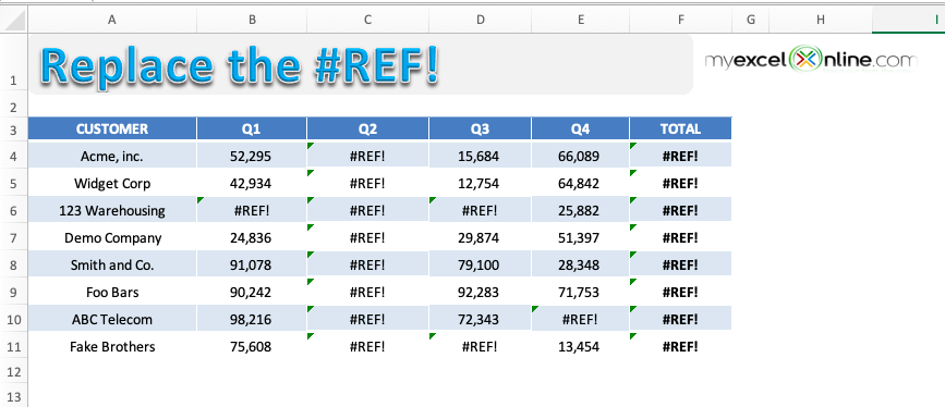
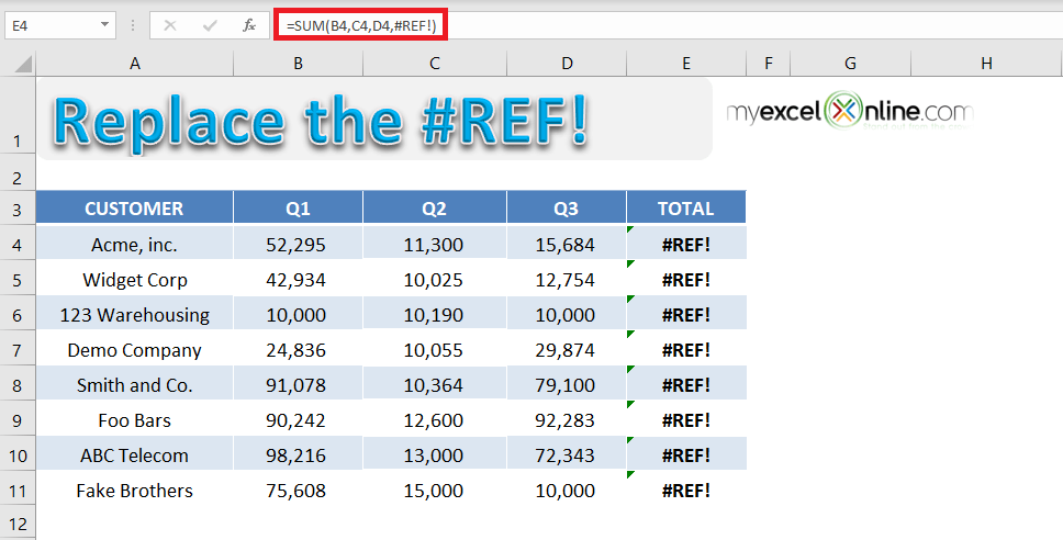
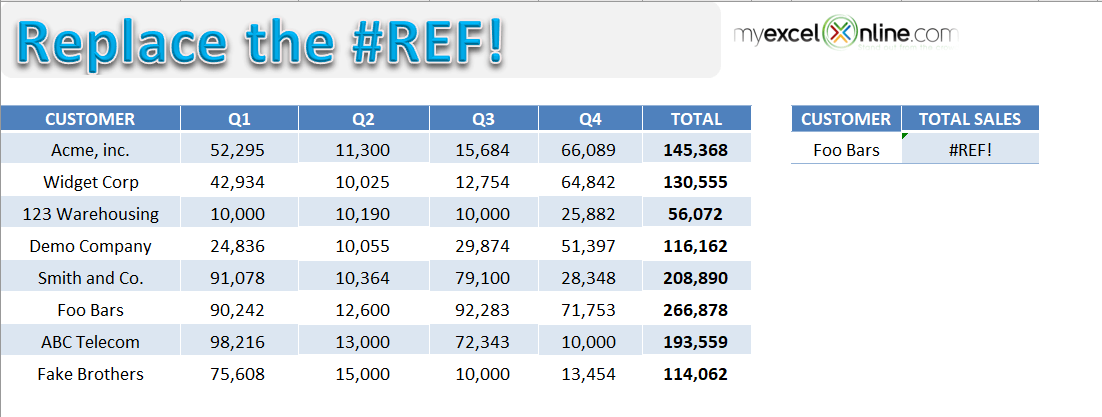
In the table below, you will spot multiple #REF! error within formulas used in the cell.
This has happened because you have deleted a range that contains an explicit cell reference within the formula used.
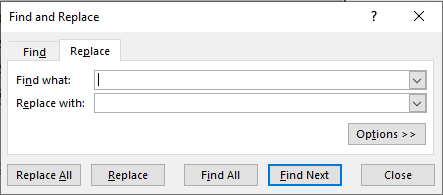
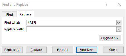
To get rid of this error message we have to select the cell(s) with this error, use the Find & Replace dialog box and do the following:
Find What: #REF!
Replace With: (Leave this blank)
Press OK and it will clear the #REF error in Excel within the formula.
Let’s look at the step-by-step tutorial below to understand how to remove #REF in Excel.
Download workbookReplace-the-REF-error-2.xlsx
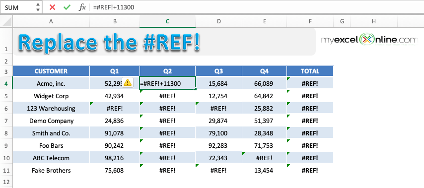
STEP 1: To check the cell containing the cell, simply click on the cell and press F2.
Here, since you have used an explicit cell reference and it was deleted, Excel is returning a #REF error.
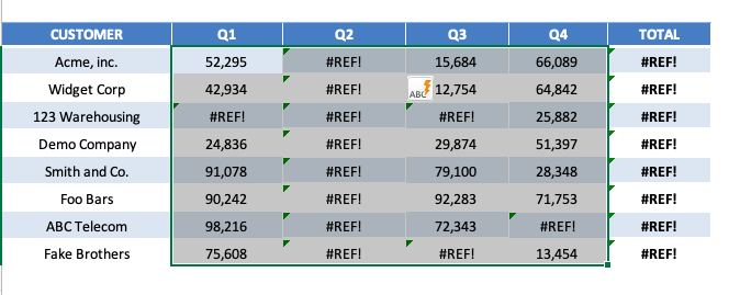
STEP 2: Highlight the table containing the errors.
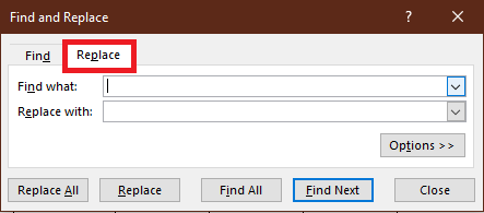
STEP 3: Press Ctrl + H to open the Find & Replace dialog box.
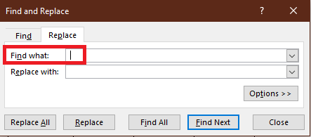
STEP 4: Under Find What, input #REF! and leave Replace as blank. This is done to replace all the #REF! error with a blank.
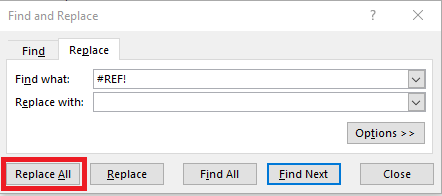
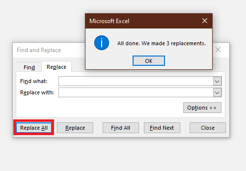
STEP 5: Click on Replace All.
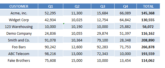
This is how your replaced data will look like:
Let’s look at another example when this error occurs due to copy-pasting the formula from other cells.
Example 2:
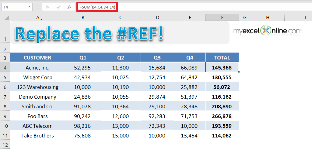
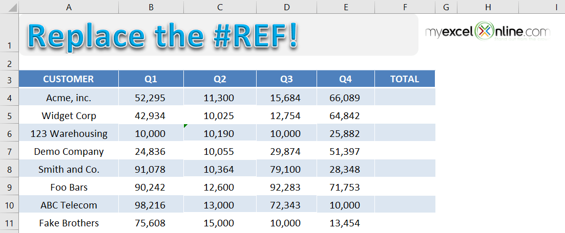
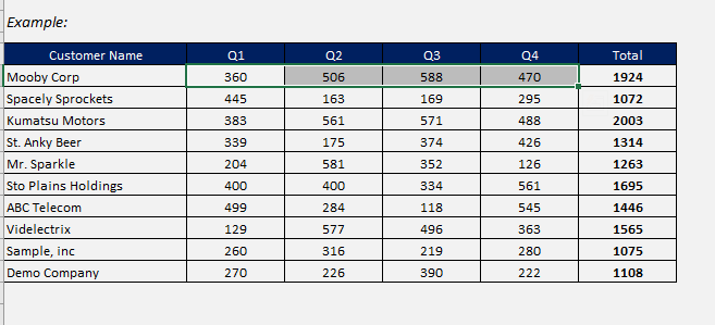
In the table below, you have sales data for different customers for 4 quarters and a sum formula used to calculate the total sales. The formula used to calculate the total sales value is =SUM(B4, C4, D4, E4).
If you try and delete Column E (Quarter 4), the sum formula will change to =SUM(B4, C4, D4,#REF!) and return an error – #REF.
This error is caused because the formula to calculate the total sales uses explicit cell reference. When one of the cell references used in the formula is deleted (here cell E4), Excel is unable to calculate the value and returns an error.
A simple fix to this problem is to use a range instead of an explicit cell reference. Let’s look at the step-by-step tutorial to learn how:
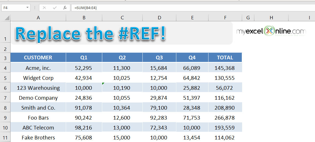
STEP 1: Use formula =SUM(B4: E4) in cell F4 and copy-paste the formula below to cells F5: F11.
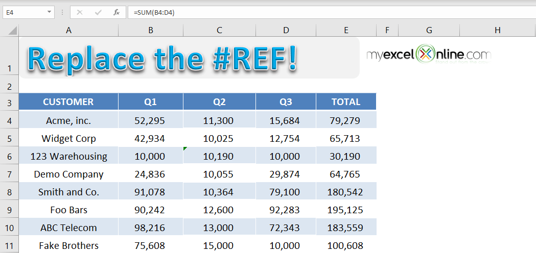
STEP 2: Now delete Column E to get the total sales for only 3 quarters.
If you change the formula from =SUM(B4, C4, D4, E4) to =SUM(B4: E4), you will no longer to vulnerable to #REF in Excel. This formula recalculates the total sales value by removing the deleted cell.
Hence, it is advised to use range while writing a formula instead of an explicit cell reference.
Let’s take a look at another example when the error occurred due to VLOOKUP containing an invalid cell reference.
Example 3:
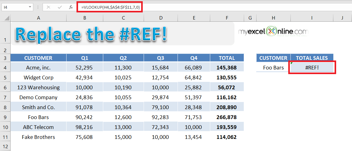
In the table below you have quarterly and total sales for different customers and using the VLOOKUP formula, you have tried to find out the total sales for the customer name mentioned.
The formula used to find the total sales for customers mentioned in cell H4 is =VLOOKUP(H4,$A$4:$F$11,7,0).
If you look into the formula used in detail, you will see that the value used to indicate the column index number is incorrect.
The arguments for a VLOOKUP function is:
- Lookup_value = The value you want to look up in the first column of the table.
- Table_array = The table from which you need to retrieve the data.
- Col_index_num = The column number in the table array from which matching value should be returned.
- Range_lookup = Value should be 1 if you want an approximate match or 0 if you want an exact match of the return value.
Excel is returning an error in this formula because VLOOKUP is looking to return a value from the 7th column but the reference $A$4:$F$11 contains only 6 columns.
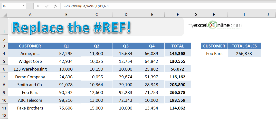
To fix this error, use the formula =VLOOKUP(H4,$A$4:$F$11,6,0).
Excel displays an #VALUE! error when the variable provided in the formula is not a supported type. This Excel error can occur because of the following reasons:
- Cell is left blank or contains hidden spaces; or
- Cell contains text instead of the number; or
- Date is treated as text, etc.
Download workbookValue-Error.xlsx
Example 1:
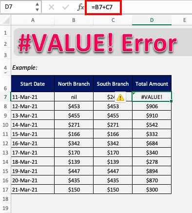
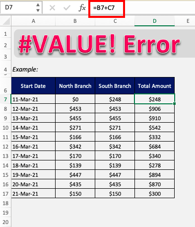
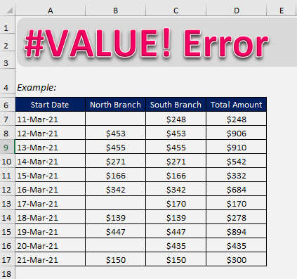
Here, we are trying to calculate the total sales amount by adding the sales achieved in both regions on different dates.
As you can see when cell D7 adds B7 and C7, it returns #VALUE! error. This is because cell B7 contains text instead of a number.
Let’s fix this!
Change the text nil to number 0.
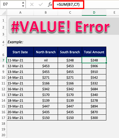
You can also use the function SUM instead of using the addition operator (+). As formulas with operators will not calculate cells with text and instead display VALUE error.
If you use functions they will simply ignore text values and calculate everything else.
Example 2:
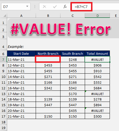
Sometimes, VALUE error will be displayed when the cell contains hidden spaces. These spaces will look like the cell is blank but in fact, it contains a space instead.
In this example, you can see even though cell B7 looks like it is a blank, value is cell D7 is displaying an error. This is because cell B7 actually contains hidden space!
There can be numerous cells that may contain hidden spaces and it may be difficult to spot and remove them.
So, follow these steps below to find extra spaces and remove them!
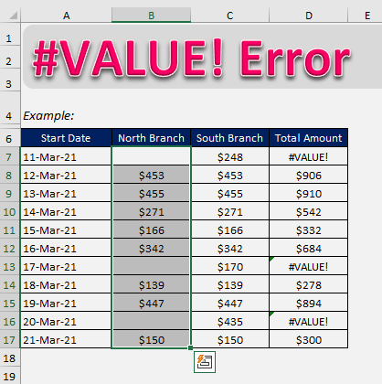
STEP 1: Select the range that contains hidden spaces.
STEP 2: Press Ctrl + F to open the Find & Replace dialog box and select Replace tab.
STEP 3: Type in an extra space in Find what field and keep Replace field blank.
STEP 3: Press Replace All button. This is remove all the hidden spaces in the selected cells and leave them blank.
All the errors will now disappear!
Example 3:
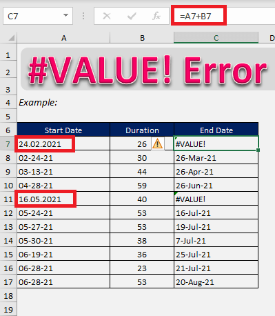
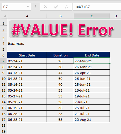
In this example, we are trying to add duration to the start day of the project in order to get the project’s end date
Here, cells C7 and C11 are displaying #VALUE! error as Excel cannot recognize the value as a date. This is because date is separated using the decimal points as delimiters.
Let’s change the delimiter from decimal point (.) to hyphen (-)!
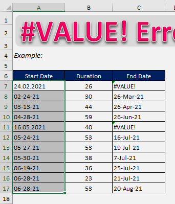
STEP 1: Select the cells containing dates.
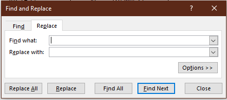
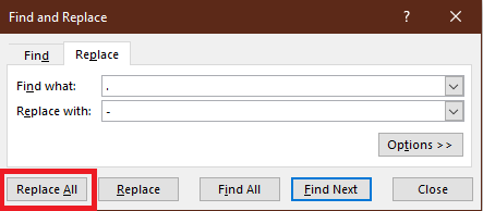
STEP 2: Press Ctrl+H to open Find & Replace dialog box.
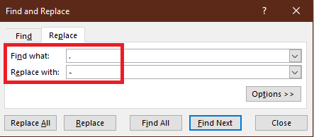
STEP 3: Type decimal point in Find What field and hyphen in Replace With field.
STEP 4: Press Replace All button.
This will replace decimal point with hyphen. Excel will now treat them as dates and make your formula work perfectly.
This error in Excel occurs when you attempt to divide a number with zero, any value equivalent to zero, or a blank cell.
download excel workbook Div-error.xlsx
Example 1:
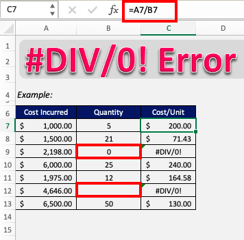
The Excel DIV 0 is a common and simple error that can easily be dealt with. To correct this error, all we have to do is make sure that the cell reference provided does not belong to an empty cell.
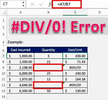
In the example below, the formula in column C is a simple dividing formula. But, cells B9 and B12 have blank cells respectively, and hence result from the division in column C returns the #DIV/0 Error.
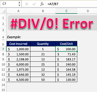
Now if we simply correct our mistakes by editing the cells in column B, the errors will disappear.
Like so!
Example 2:
In most cases, the referenced cell should actually contain the value 0 or be empty. A simple solution to this will be to use an IFERROR formula and get rid of the error message.
We can design the IFERROR formula in such a way that it either returns 0 or any value as desired if the result of the original formulas occurs to be an error.
What does it do?
It returns a value that you set if a formula has an error
Formula breakdown:
=IFERROR(Value, Value if Error)
What it means:
=IFERROR(The Formula, What do you want to show if The Formula has an error?)
If you have a calculation that results in an error like, #N/A, #VALUE!, #REF!, #DIV/0!, #NUM!, #NAME?, then you can clean it up by using the IFERROR function which allows you to replace the error it with a custom text.
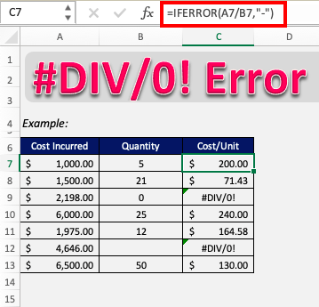
In this example, cell B9 contains 0, and cell B12 is empty. The corresponding cells C7 and C12 are thus displaying #DIV error.
Let’s wrap the division formula around the IFERROR formula and see what happens.
=IFERROR(A7/B7,”-“)
Here, we specified in the formula that if the value in cell C7 returns an error, it will be replaced by our custom text – hyphen (-).
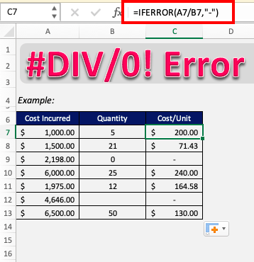
Apply the same formula to the rest of the cells by dragging the lower right corner downwards.
Hence as cells B9 and B12 had blank or 0 values, the corresponding cells in column C should produce an error but IFERROR changes it to display hyphen (-).
This error occurs when the range provided in the formula is not valid and you have provided an incorrect character instead of the required character in the range.
This can be mainly due to two reasons :
- Wrong input instead of a colon (:)
- Wrong input instead of a comma (,)
download excel workbook Null-error.xlsx
Example 1:
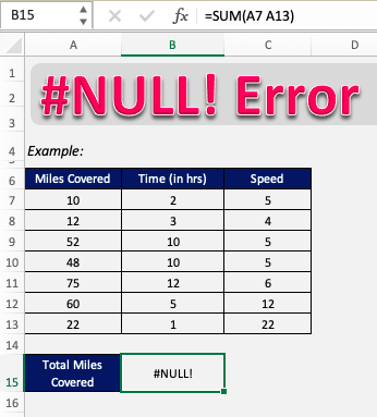
Sometimes in a formula, where there is supposed to be “:”(colon), you might have entered space. This can be the result of the error that we are getting as shown below.
In the formula bar, we can see that instead of =SUM(A7:A13), it is entered as =SUM(A7 A13), which is the cause of the error.
So to correct this, we have to replace that space with a colon(:).
Like so! As the typo has been corrected, the error has been removed and the formula is returning the correct value.
Example 2:
Sometimes in a formula, where there is supposed to be “,”(comma), you might have entered space.
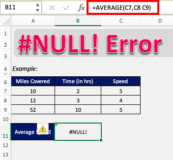
In this example, we are trying to calculate the average speed in cell B11 based on the 3 entries mentioned in rows 7, 8, and 9. The formula used is:
=AVERAGE(C7,C8 C9)
This can lead to an error that we are getting as shown below:
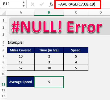
Here, instead of =AVERAGE(C7,C8 C9) you should enter the formula as =AVERAGE(C7,C8,C9).
There should have been a comma between C8 and C9 but instead, there has been a typing error and instead of the comma, space was inserted.
Simply removing the space and adding the comma rectifies this error.
There are various formulas in Excel that populate results in multiple cells. It is termed as actually spilling the data into the neighboring cells.
The different scenarios when you can encounter this error are:
- Spill range isn’t blank
- Spill range contains merged cell
- Spill range is too big
- Spill range in a table
Excel is unable to fix these errors and display the output. Since the formula cannot populate all the cells it is supposed to, the first cell where the formula is entered shows the #SPILL! Error.
download excel workbook SPILL-error.xlsx
Example 1: Spill range isn’t blank
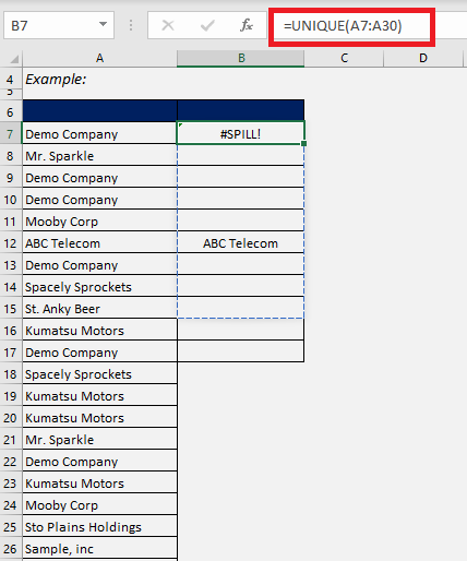
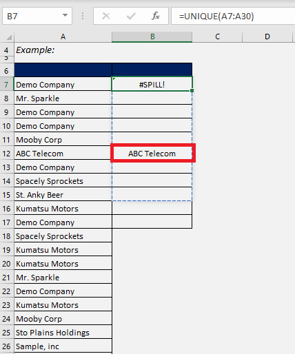
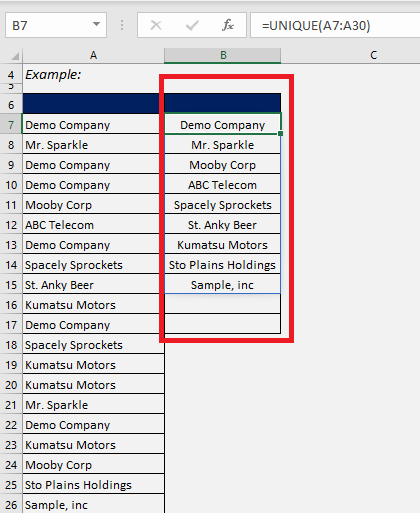
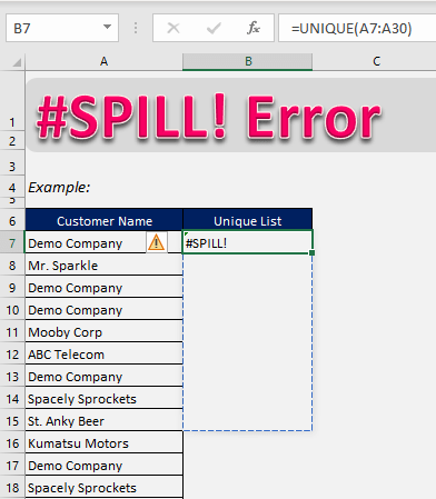
You want to find a unique list of customer names stated in column A using the UNIQUE function in Excel. But, Excel returns a #SPILL! error instead.
This is because the output range already contains data and Excel cannot overwrite it and populate the desired result.
Solution:
Simply, clear any contents from the output range and you are good to go!
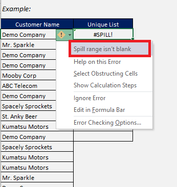
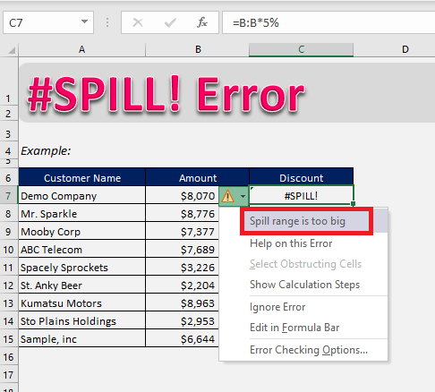
The spill error can have multiple causes. To understand the root of this problem, click on the small yellow! warning sign next to the error. It shows the cause of the problem.
Most commonly it is caused because there is a cell containing some value, but it needs to be populated by the formula. Removing the value in all such cells will remove the “blockage” and, in turn, the error.
Simply, clear any contents from the output range and you are good to go!
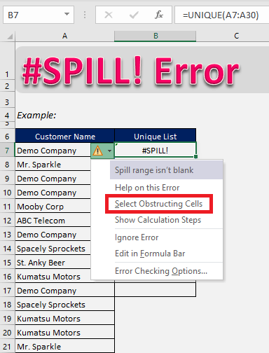
There can be times when you get the SPILL error but you are unable to spot the cell that contains unwanted data.
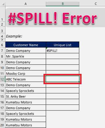
Click on Select Obstructing Cells and it will take you to the cell that is creating the problem.
This is useful when you have hidden spaces and you are unable to find them.
Example 2: Spill range contains merged cells
SPILL error can also occur when the result range contains the merged cells.
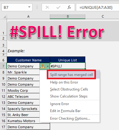
In this example, you can see the spill range i.e. B7:B15 is empty but still, Excel returns #SPILL error.
To be sure of the reason, let’s click on the yellow warning sign and see what it says – Spill range has merged cell.
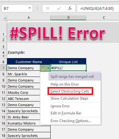
Now, click on Select Obstructing Cells and it will take you there.
Go to Home > Merge & Center to unmerge the cells.
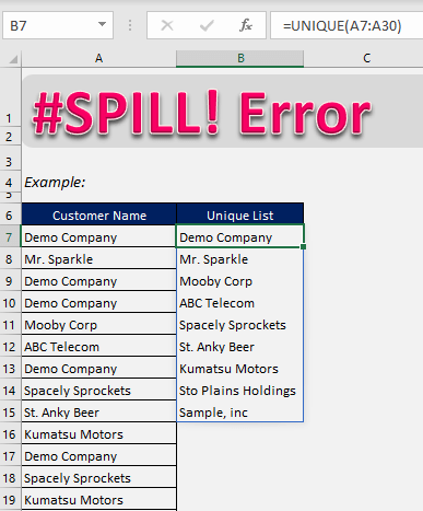
The result is now visible and the error disappears!
Example 3: Spill range is too big
This error occurs when the output range is too big and the result goes beyond the boundary in Excel. There isn’t enough space to display the result.
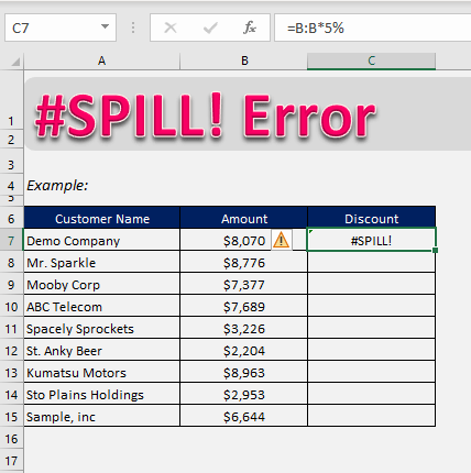
In this example, we are trying to calculate the discount given to the customers based on the sales amount. Column C is used to get 5% of the sales amount.
As you can see, Excel is again and producing a SPILL error and this time it is because the range is too big.
Here, Excel is trying to multiply each cell in Column B by 5% and produce a million results. It will spill the result in Column C starting from cell C7 but it will reach the end of Excel.
Hence, the error!
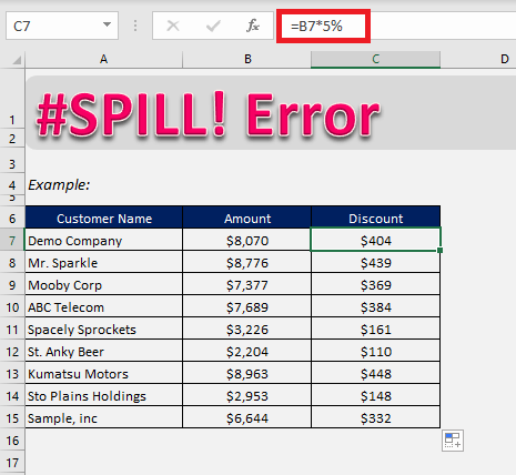
To solve this, simply replace the column with the relevant range and copy the formula to the output range.
Example 4: Spill range in a table
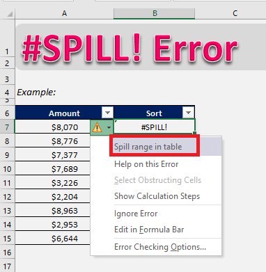
Excel tables do not support spilled array formulas. If you try to insert an array formula in an Excel table, it will return a #SPILL error.
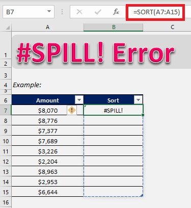
In this example, we are trying to sort the amount mentioned in Column A in ascending order using the SORT function. It will return a dynamic array as a result in column B.
Unfortunately, we are getting a #SPILL Excel error. This is because range A7:B15 is in fact saved as a table in Excel and dynamic functions do not work within Excel tables.
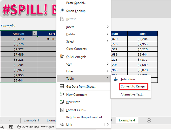
We can easily convert it into a range for our SORT function to work properly.
To do so: Right Click on any cell in the Table range > Select Table > Select Convert to Range.
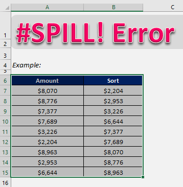
This will convert the table to range and now all array functions will work perfectly as shown below!
The #NAME? Error is a fairly common one that even seasoned Excel professionals can face. It occurs when there:
- Spelling error in Formula name
- Spelling error in Cell Range
- Spelling error in Named Range
- Text entered without quotes
download excel workbookName-error.xlsx
Example 1: Formula Name
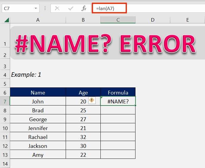
When entering the name of the formula if the name is misspelled, then that can lead to the occurrence of this error.
In the above example, you can see that instead of writing =LEN(A7), we have typed =lan(A7). There is an error in the formula name, leading to the problem.
Now you can see, simply correcting the name removes the error displayed.
The best way to not get #NAME excel error is to choose the formula in the drop-down list while typing the name of the formula. This makes sure that the formula name is not misspelled.
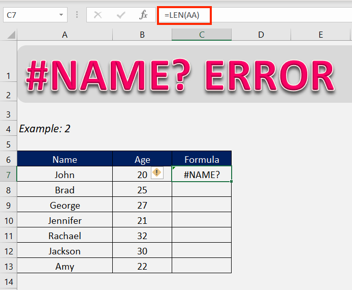
Example 2- Cell/Range name
When entering a formula that references a certain cell or range, misspelling the name of the cell or range can lead to this error.
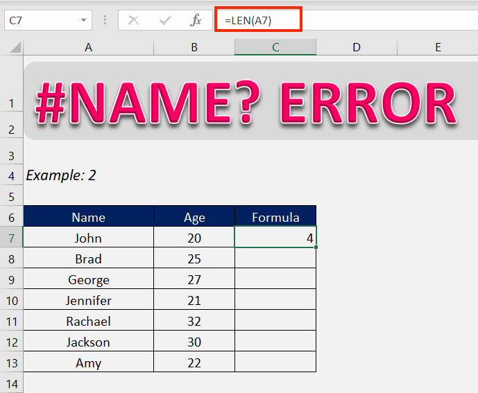
Here we can see that the name of the cell is misspelled. Instead of =LEN(A7), it is typed as =LEN(AA).
To rectify this, simply type in the correct cell name.
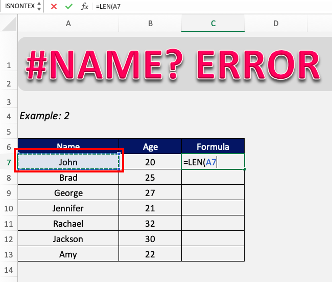
A better way of avoiding the error is to select the cell when referencing in the formula. This will lead to always entering the correct cell name.
NAME error in Excel can occur when entering a range. Check and correct the range name or select the entire range when entering the formula to rectify the error and prevent it.
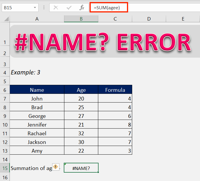
Example 3- Named range
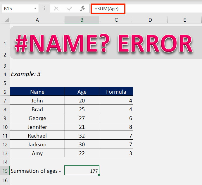
There can be particularly important ranges in your workbook that you have assigned a name to. When referencing this range in a formula, misspelling it can lead to the #NAME error in Excel.
Here we can see that the range referenced to in the formula is spelled agee when the correct name is Age.
Correcting the name of the range or simply selecting the range when referencing it in the formula will correct this error.
Example 4- Text without quotes
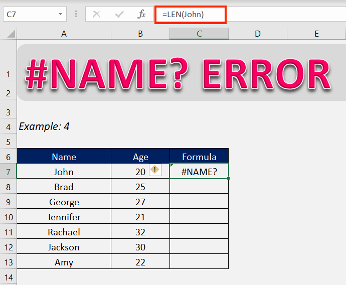
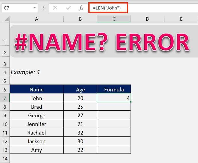
Wherever a text is entered into a formula, it should be entered in quotes. When a text value is not confined between quotes, Excel reads it as either a formula or a named range/table.
If there is no formula or named range in your workbook that matches the text written in the formula, Excel will return the #NAME? Error.
Here we can see the text entered in the formula is not in quotes and hence Excel is returning it as an error.
Now that the text is written in quotes, Excel is returning the correct value of the formula.
Excel shows the #NUM! Error when values in formulas are invalid. It basically means that the calculation cannot be performed due to limitations or errors.
This can be due to the fact that the number is too big or small, impossible calculations, or when the data type is not supported in the argument.
download excel workbookNum-error.xlsx
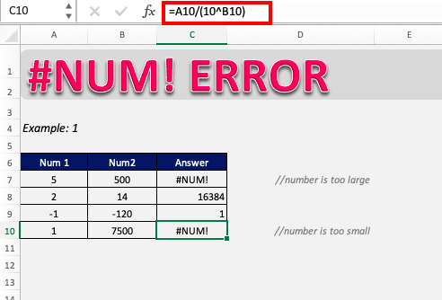
Example 1 – Number size
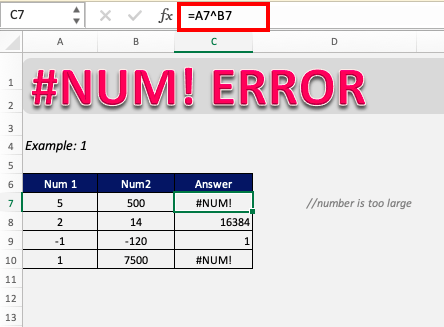
Excel has a limitation to the size of the number that it can display. If you enter a number is too large or too small,you will get Excel #NUM Error.
As you can see, in cell C7 we are trying to multiply 5 by itself 500 times. The result will be a really large number that Excel is unable to display. Hence. it returns NUM Excel.
In cell C10, we are trying to divide 1 by 10^750. Since this will be a very small number Excel cannot perform calculations and hence returns #NUM error.
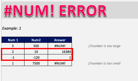
Excel is not able to show these values because of its inherent limitations. As shown, other smaller values are calculated and shown in C8 and C9.
Example 2 – Impossible calculations
Excel returns the #NUM! Error when it is faced with a calculation that is impossible to do.
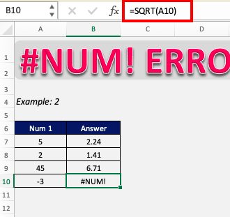
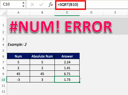
As you can see, the square root or log of the positive numbers has results but the square root or log of the negative numbers is impossible to calculate.
In this example, we are trying to find the square root of -3.
Since we are trying to calculate the square root of a negative number, we will get #NUM error in Excel. In this particular case, you can rectify this issue by taking the absolute value of the number.
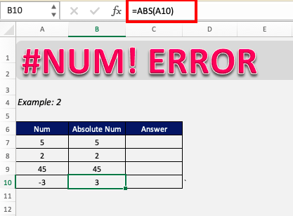
ABS function returns the absolute value of a number. It converts negative numbers to positive numbers and keeps the positive numbers unaffected.
Including the ABS function into the formula uses the absolute value of the number in column A, so now Excel can calculate the number and return a valid answer.
Example 3 – IRR function not working
Excel might show the #NUM! error when using IRR function because of either one of the two reasons:
- Cash flow does not contain at least one negative and one positive value.
- Formula can’t find a result.
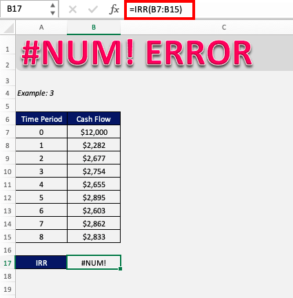
In this example, Excel results a #NUM error instead of proving a value.
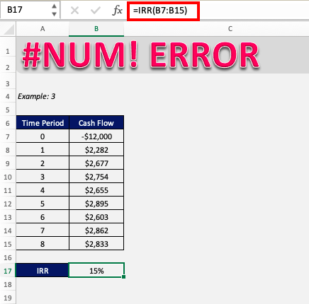
This is because the cash flows provided in the range (B7:B15) are positive and IRR requires at least one negative value as the initial cost of business.
Initial payments are provided as negative value indicating outflow of cash and income payments are represented by positive values. Once you have incorporated this, the function will provide the correct result!
IRR function can also display #NUM! error when the function iterates and can’t find a result after several tries.
To overcome this, you can increase the maximum number of iterations that Excel performs to get a result.
To increase the number of iterations:
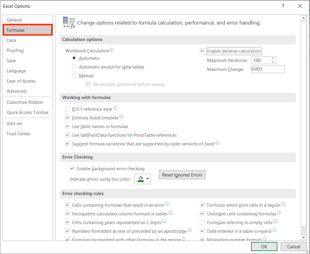
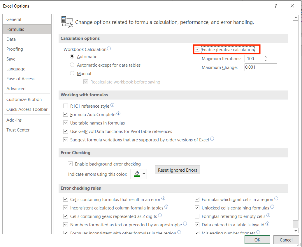
STEP 1: Go to File > Options > Formulas to arrive at the window below
STEP 2: Under the Calculation options group, check the Enable iterative calculation box.
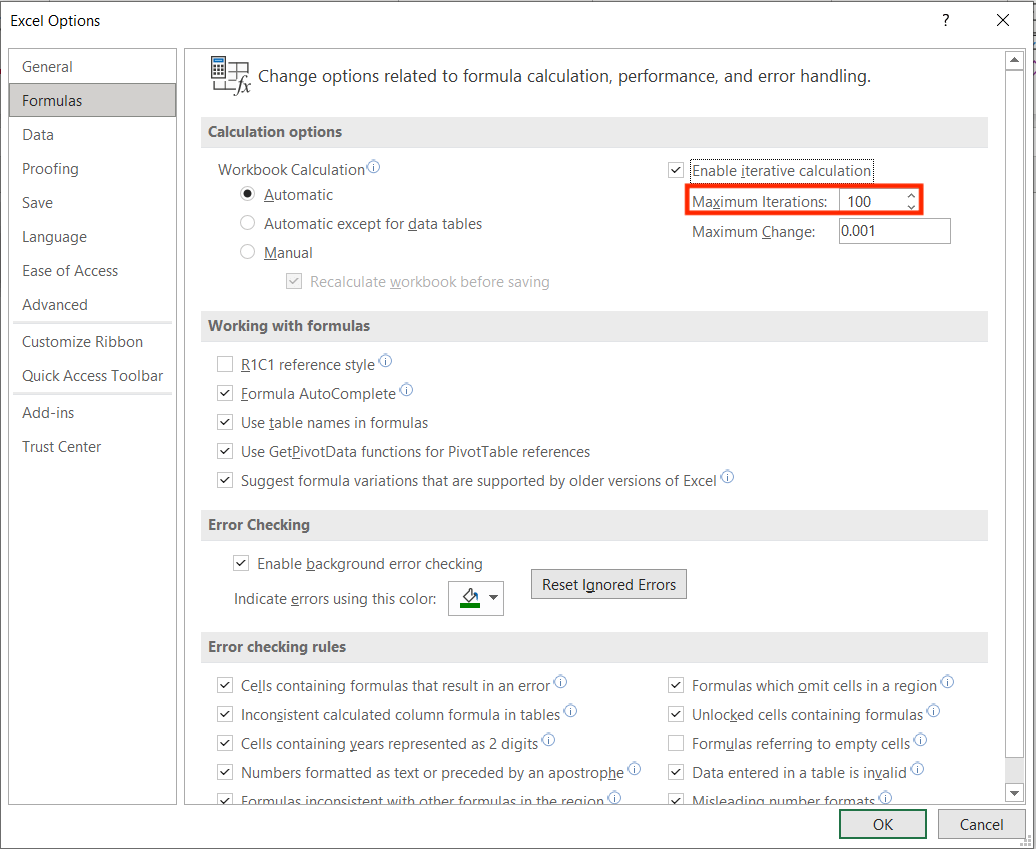
STEP 3: In the Maximum Iterations box, type the number of times you want Excel to recalculate.
The higher the number of iterations, the more time Excel needs to calculate a worksheet. Increasing this can help give a result to your calculation.
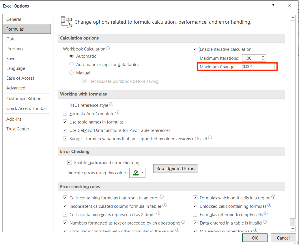
STEP 4: In the Maximum Change box, enter the amount of deviation that you are willing to accept between the calculation results.
The smaller the number, the more accurate the result. Increasing this can help give an approximate answer to your calculations.
Visual and Navigation Issues
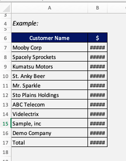
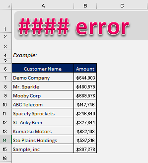
Sometimes in Excel, especially when you open a file on which you have worked before, there may be some cells that are filled with “#” signs.
Excel #### error is a very simple but common issue that can easily be solved. There are three simple ways to tackle this problem.
download excel workbook Hash-Error.xlsx
Method 1:
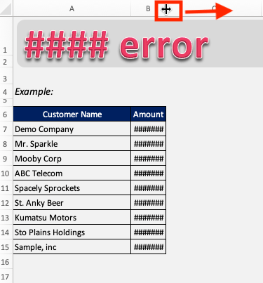
Taking your cursor to the divider between two column heads, the cursor will change into a dragger. Dragging the column head divider will change the width of the column.
Now you can increase the width to fit all the characters of the cell, or to any width that you want.
Method 2:
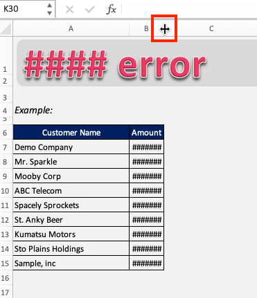
Simply double-clicking on the rightmost edge of the column head, that contains the cell filled with # marks, will autofit the column so that it perfectly adjusts and shows all values in cells.
It will adjust to the length of the longest cell in the column.
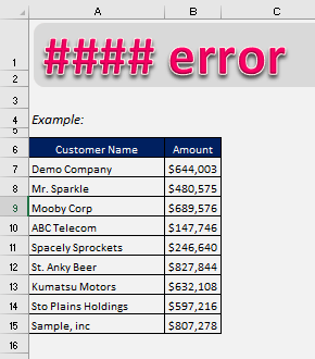
Upon applying the above steps, your values will then be visible as shown.
Method 3:
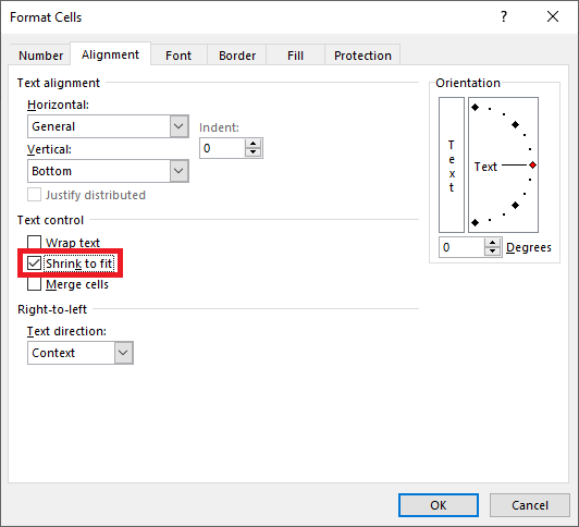
Another way to overcome this problem is auto-shrinking text to fit in the column width. To accomplish this, follow the steps mentioned below:
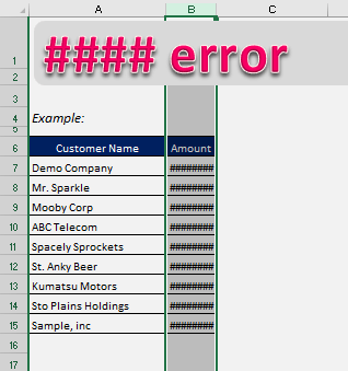
STEP 1: Select the column that shows #### error.
STEP 2: Click on the Home Tab.
STEP 3: Click on expand icon at the bottom right corner of the Alignment group.
STEP 4: Check the Shrink to fit box in the Format Cells dialog box.
Upon applying the steps, the size of the text will be reduced to fit in the column width and it will look like this:
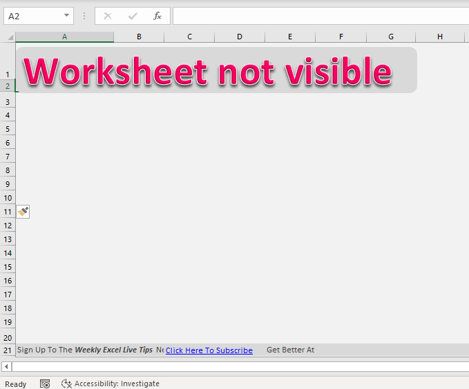
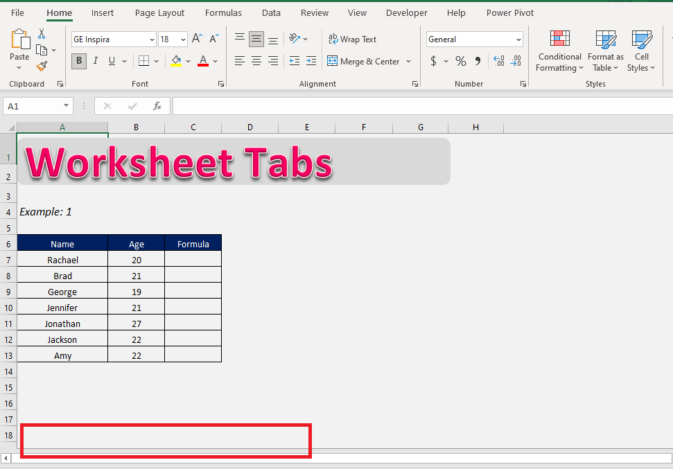
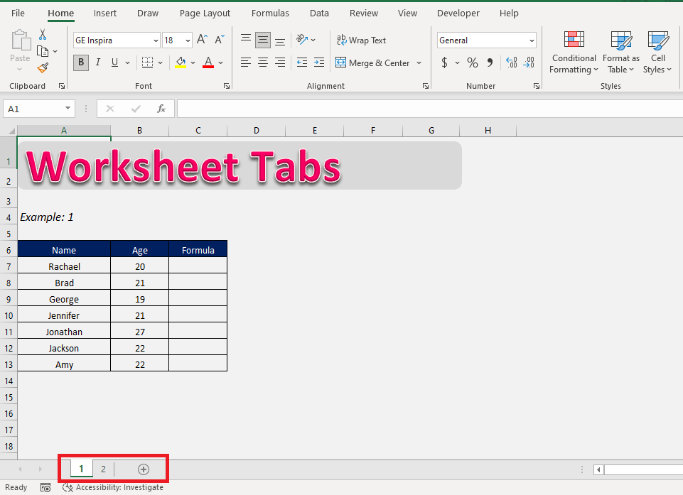
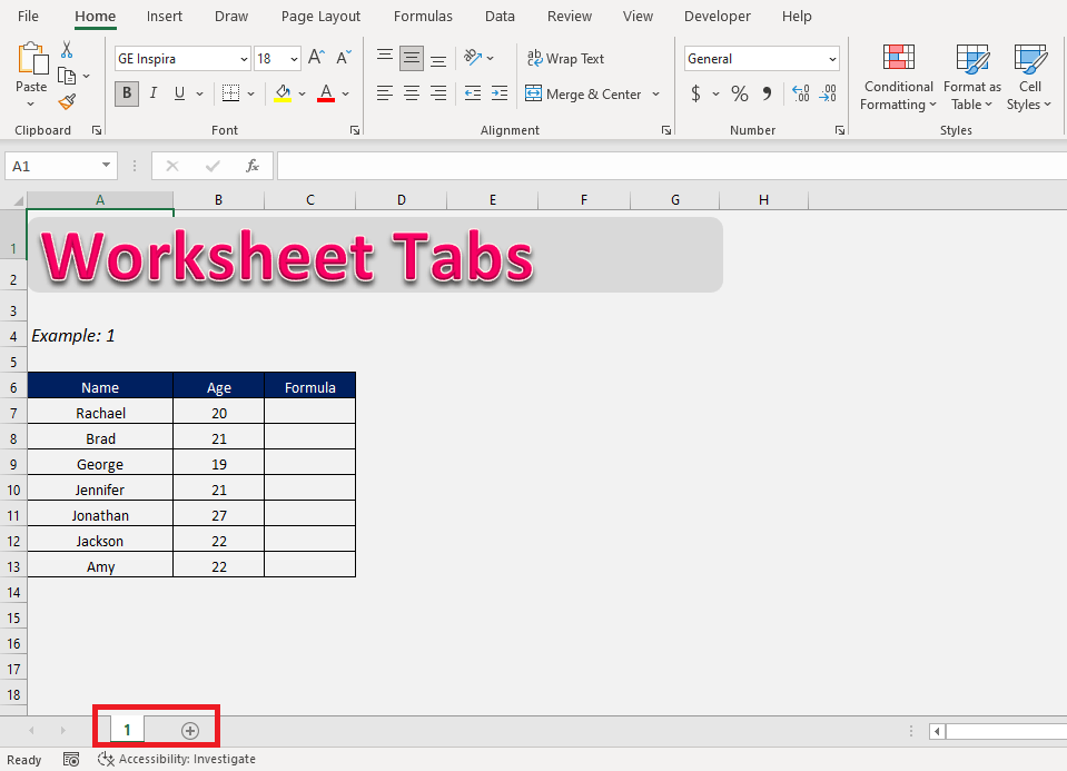
A common issue faced while operating on Excel is that your worksheet tabs (shown at the bottom left) are not visible to you.
This is a simple settings problem that can be easily undone.
download excel workbook Worksheet-tabs.xlsx
Problem 1:
Ever encountered this situation where you open your workbook and said “Where are my worksheet tabs ??”.
A common issue faced while operating on Excel is that all the worksheet tabs, which are shown at the bottom left of the window, are not visible to you.
This is a simple settings problem that can be easily undone.
Solution:
Just follow the steps below to learn how to display the missing worksheet tabs:
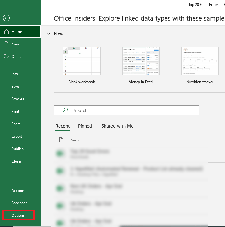
STEP 1: Go to Files
STEP 2: Click on Options
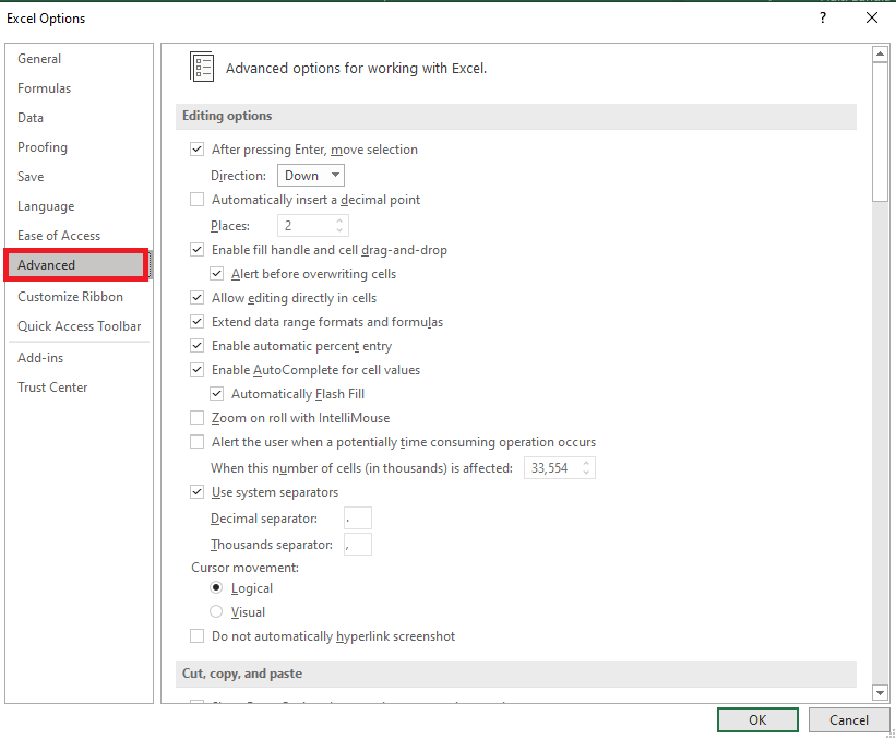
STEP 3: Click on Advanced
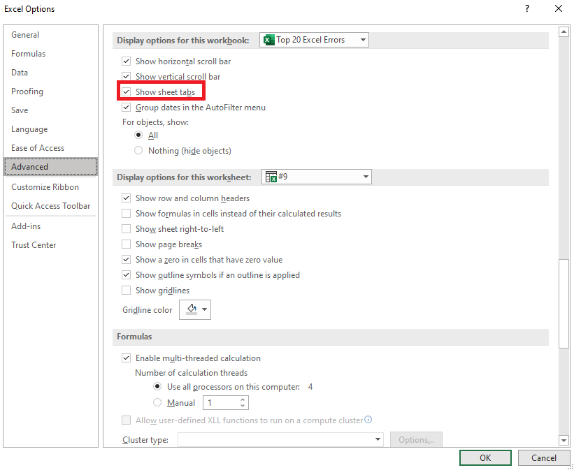
STEP 4: Under the Display options for this workbook, check Show sheet tabs.
Now your sheet tabs will be available! Now you can easily navigate through the entire workbook, and work on all sheets.
This is what to do when worksheet tabs go missing and you are unable to switch between different tabs!
Problem 2:
It can also be that some of your worksheets might be hidden, hence you will not be able to see them in the worksheet’s tab.
Here, we actually have two worksheets, but one of them is hidden.
To show the worksheet tabs:
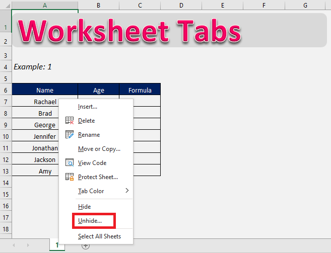
STEP 1: Right-click on any visible tab and select Unhide.
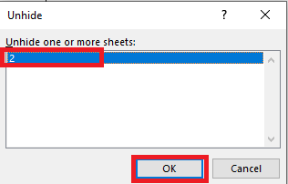
STEP 2: Select the tabs you want to unhide and press on OK.
Now both the worksheets will be visible to you on the worksheet’s tab.
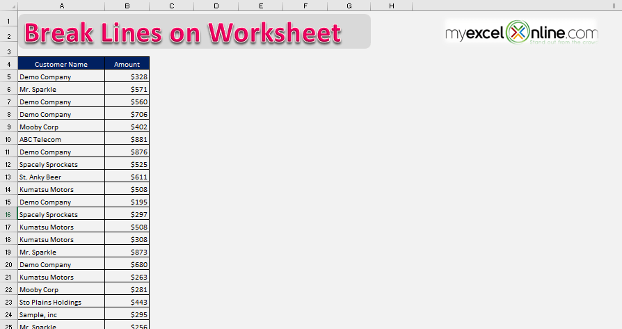
10. Break Line displayed on the Worksheet
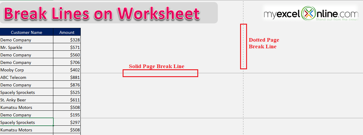
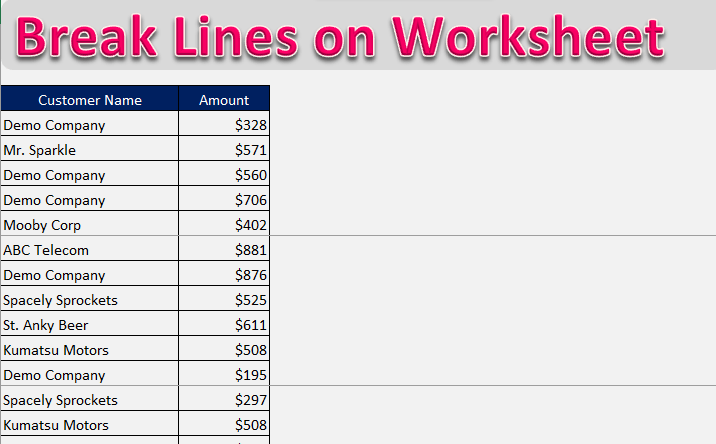
While working on Excel, sometimes you may see solid or dashed break lines added and the worksheet is divided into multiples pages.
The solid lines are manually inserted ones whereas the dashed line is automatically generated.
These are basically page breaks inserted in Excel for printing purposes! They may be useful when you are trying to print a document but other times are just visually distracting.
You may want to remove these lines before presenting your worksheet to someone!
In this article, we will cover the different ways to remove lines from the worksheet:
- Solid Page Break Line
- Dotted Page Break Line
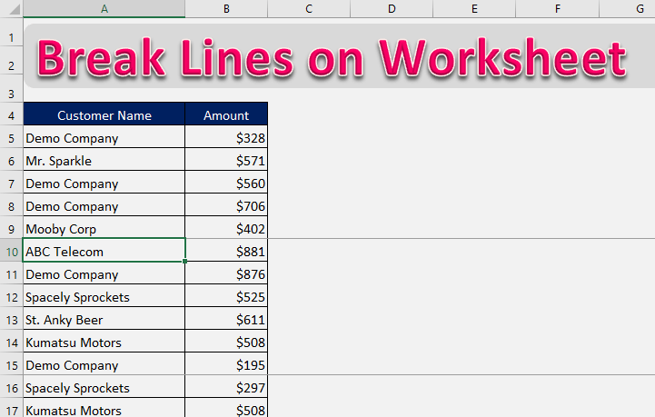
In this screenshot, we have two solid lines inserted in the worksheet.
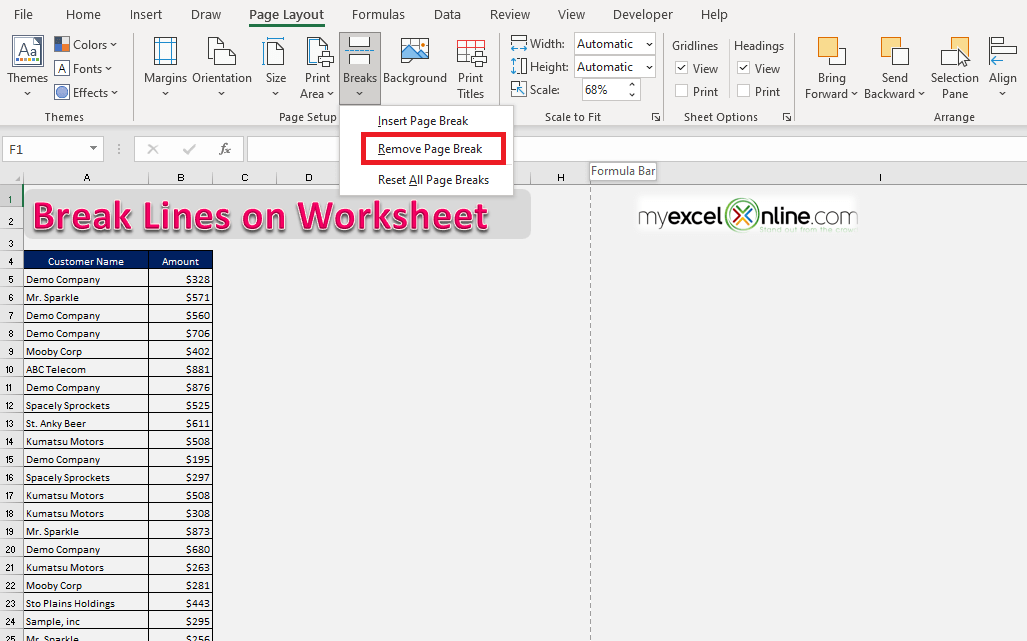
These are manually added page breaks and can easily be removed by following the step-by-step tutorial below:
STEP 1: Select the cell just below the page break line.
STEP 2: Go to the Page Layout tab.
STEP 3: Click on Breaks in the Page Setup group.
STEP 4: Click on Remove Page Break.
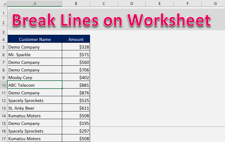
This will remove the page break between row 9 and row 10!
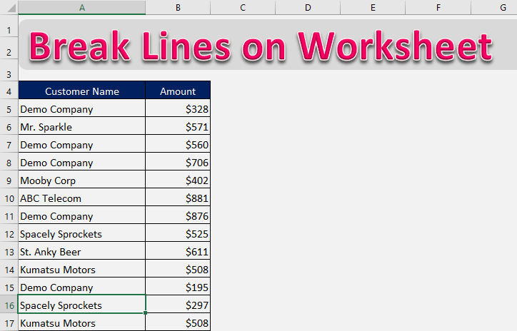
Now, follow the same steps to remove the solid line between rows 15 and 16.
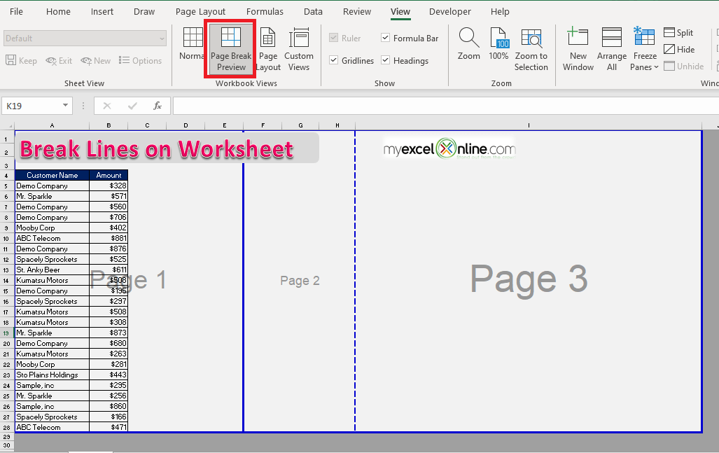
When you select the Page Break Preview in Excel, the dotted and solid lines dividing the worksheet into different pages become visible.
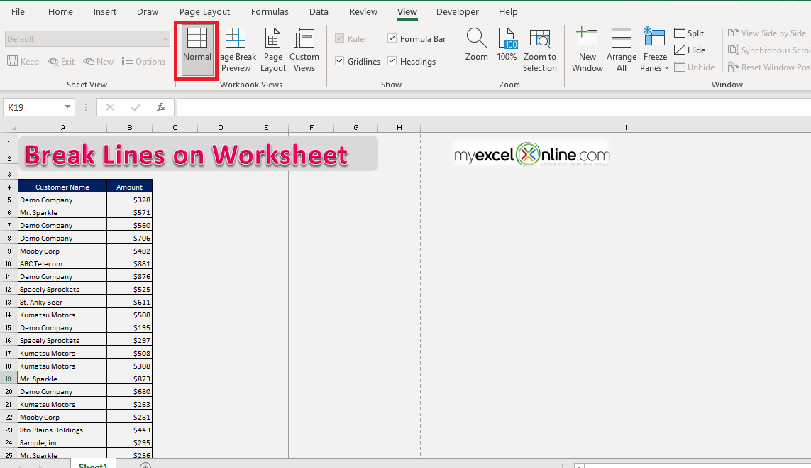
Now when you go to View > Normal, the page preview is returned to normal but the lines still visible.
To remove the solid lines, follow the steps mentioned below. But, this will not remove the dashed lines.
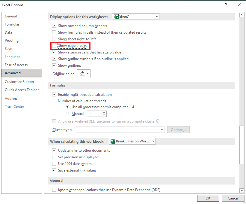
To remove the dashed line, follow the steps below:
STEP 1: Select the File tab.
STEP 2: Click Options from the menu on the left side
STEP 3: In the dialog box, click on Advanced from the left panel
STEP 4: Under display options for this worksheet, uncheck Show Page Breaks.
This will remove the dashed lines from the worksheet as well!
11. Clicking Enter key goes to the cell underneath
In general, when you press enter in Excel it solidifies the work done in a cell but it automatically takes you to the cell below the one you were working on. If this is a hindrance to you, you can easily change it.
Solution:
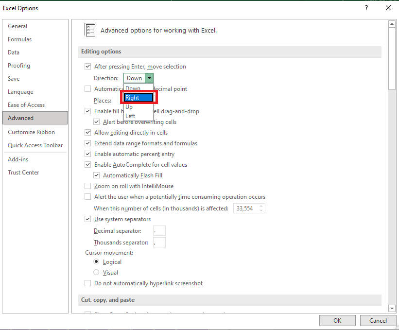
To alter the direction in which Excel files after pressing enter, follow these steps:
- Click on the File tab on the ribbon above
- Click Options from the menu on the left side
- In the dialog box, click on Advanced from the left panel
- Under Editing Option, Select After Pressing Enter Move Selection, and from the drop-down menu the choose the direction in which you want Excel to move.
Now Excel will move in the direction you want after pressing enter. Now you try it!
12. Show column headers on each page when printing
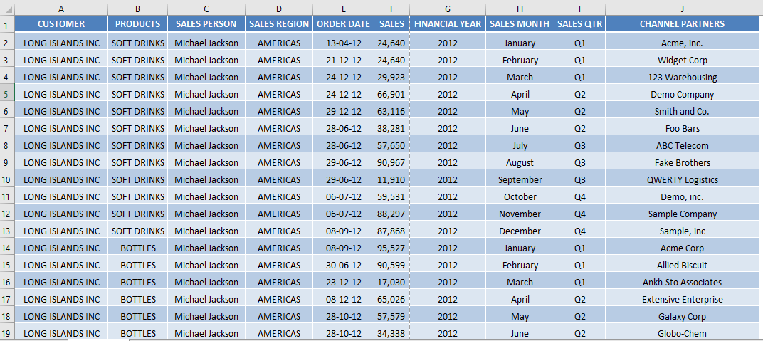
If you have a large data file with headers on the top, you can freeze the columns to easily view the entire table without losing sight of the headers.
But the freeze feature will not be applied when you try to print the file.
To print Excel header row on every page, you can try one of the following methods as per your requirement:
- Repeat row on every page
- Repeat column on every page
- Print row numbers and column letters
Example 1: Repeat row on every page
If you have a large worksheet that spans over multiple pages, you can easily print the first row of the data as headers in Excel on every page.
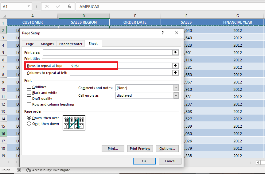
Follow the steps below to print a row of every page:
STEP 1: Go to Page Layout tab > Select Print Tiles
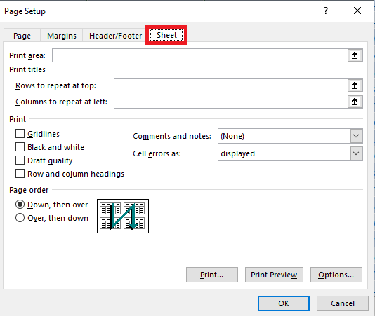
STEP 2: In the Page Setup dialog box, select Sheet.
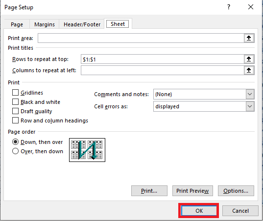
STEP 3: Select the collapse dialog box and pick the row you wish to repeat.
STEP 4: Click OK.
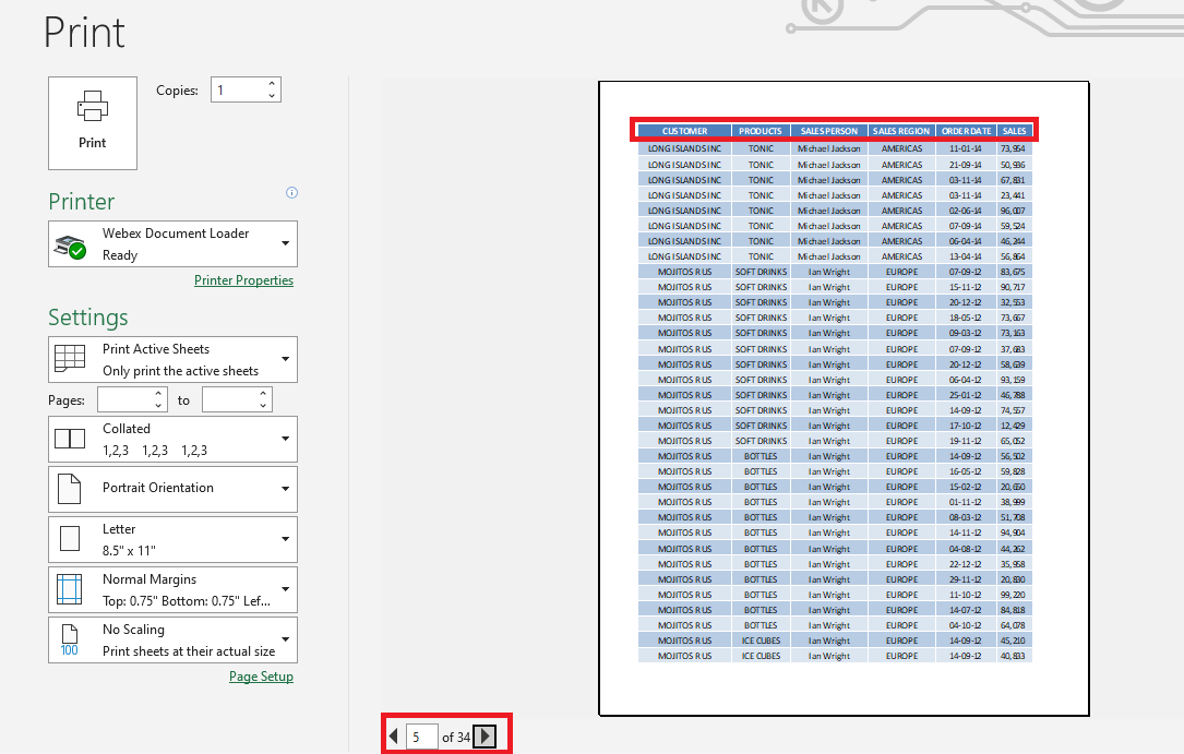
STEP 5: Press Ctrl + P to open Print Preview.
As you can see we are on page 5 but the 1st row is still visible!
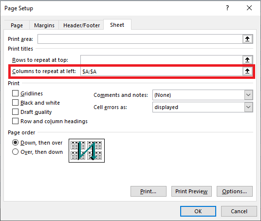
Example 2: Repeat Column on every page
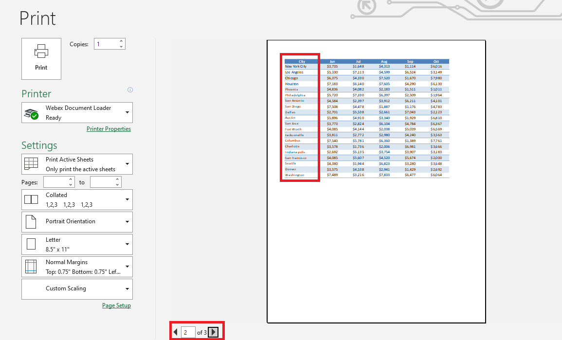
When your Excel worksheet has multiple columns and is spread across several pages, you can fix the first column.
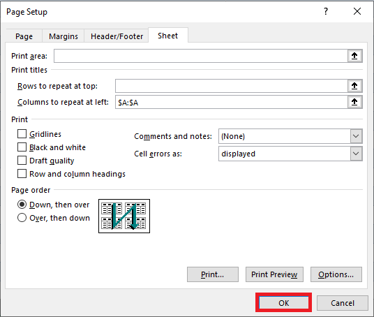
Follow the steps below to fix the first column when printing:
STEP 1: Go to Page Layout > Select Print Tiles
STEP 2: In the Page Setup dialog box, select Sheet.
STEP 3: Select the collapse dialog box and pick the column you wish to repeat.
STEP 4: Click OK
And it’s done! Column A is still visible when you go to page 2.
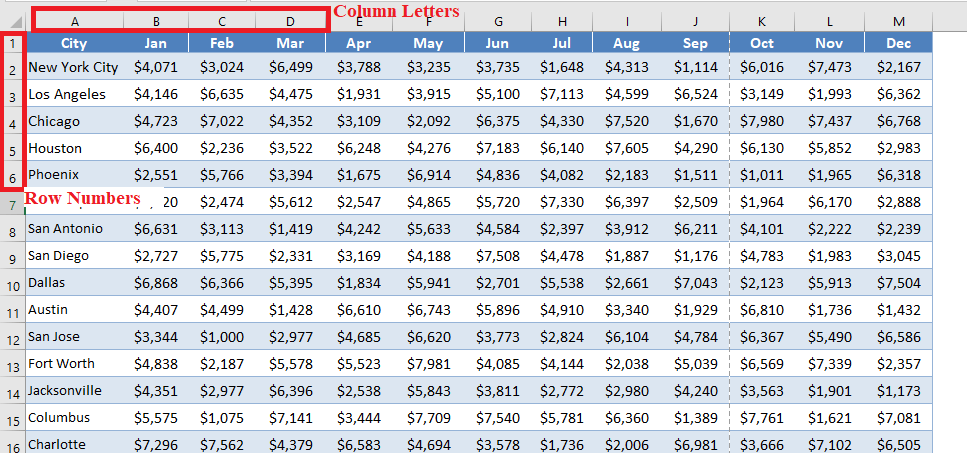
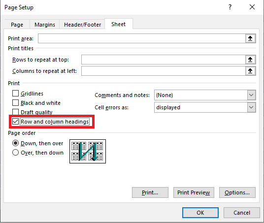
Example 3: Print row numbers and column letters
Excel denotes the worksheet’s columns as letters (A, B, C, etc) and rows as numbers (1, 2, 3, etc). But when you try to print your worksheet, it is not visible at all.
You can easily print numbers and column letters by following the steps below:
STEP 1: Go to Page Layout > Select Print Tiles
STEP 2: In the Page Setup dialog box, select Sheet.
STEP 3: Check Row and column headings
STEP 4: Click OK.
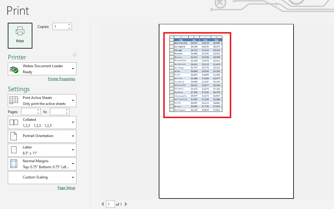
STEP 5: Press Ctrl + P to view Print Preview.
The row numbers and column letters will be displayed in the print preview section!
Operational Issues
13. Not using Quotation Marks for Text in Formulas
When writing formulas, Excel will identify a text only if it’s written within quotation marks. Excel extracts anything written within the quotation mark as text and discards the quotation mark.
Let’s use a formula to use to help better understand the use of quotation marks while writing a formula!
Download workbookQuotation-Mark.xlsx
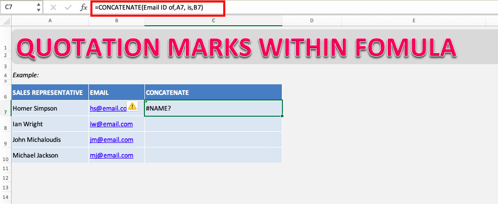
In this example, we have tried to insert text like “Email ID of” and ” is” but Excel is returning an error. This is simply because Excel will not consider text if it is not provided within quotation marks in a formula.
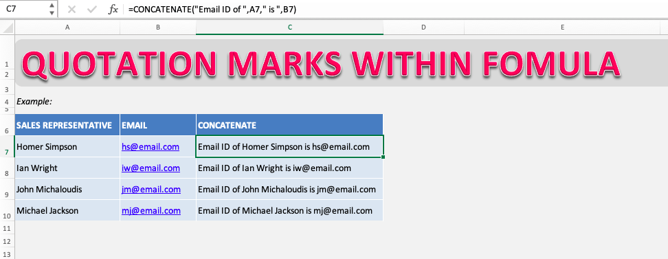
Now, put them within quotes and try using this formula again.
And Voila, the error is resolved and we can now insert custom text within the formula easily.
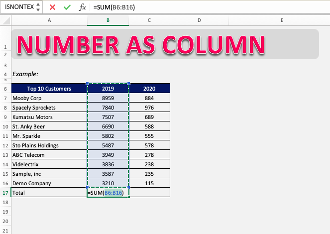
14. How to Use Numbers as Column Headings
You may have faced a situation when you need to use numbers as column headings in the table. But, when you put in digits as heading, Excel will treat it as a number and not text.
As a result, when using auto sum or other similar features the heading will also be included with other values.
Download workbookNumber-as-Column-Header.xlsx
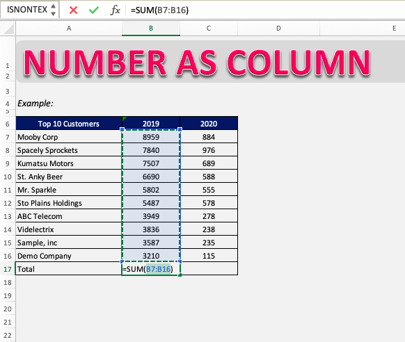
This is not the result you were expecting! Let’s fix it by forcing Excel to consider the number as text.
To do that, simply add a ‘ symbol in front of the number and it will be treated as text.
See, it is that simple! Try it now!
15. Unable to Directly Edit the Cell
If you are unable to edit data entered in your Excel worksheet and you are not sure how to fix it, you have come to the right place. There are several ways in which you can easily enable editing cells and learn how to edit cells in Excel.
- Excel file is read-only
- Excel worksheet is locked
- Editing in cell disabled in Excel
Example 1: Excel file is read-only
You may not be able to edit any cell in Excel because the Excel worksheet has been saved as read-only. This will force Excel to keep the worksheet in view mode and you can make no changes in the file.
To fix this, simply press the Enable Editing button on the top of the Excel worksheet.
On you press that button, you can easily edit any cell in Excel.
Example 2: Excel worksheet is locked
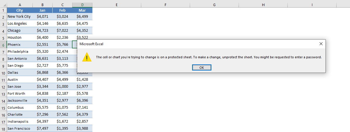
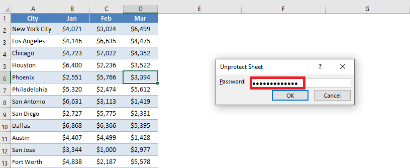
Another reason why you may not be able to edit cells is that your Excel worksheet has been locked. You have to unprotect your worksheet first and then you can make changes in your file.
To make changes in Excel, follow the steps below:
STEP 1: Go to the Review tab
STEP 2: Click on Unprotect Sheet
STEP 3: Enter the password in the unprotect sheet dialog box and click OK.
The password for this worksheet is “myexcelonline”.
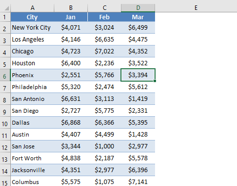
This will unprotect the sheet and you will be able to make the edits you want.
Can’t remember the password that you had used to lock your Excel file? Click here to learn how to unprotect active worksheets using macros in Excel.
Example 3: Editing in cell disabled in Excel
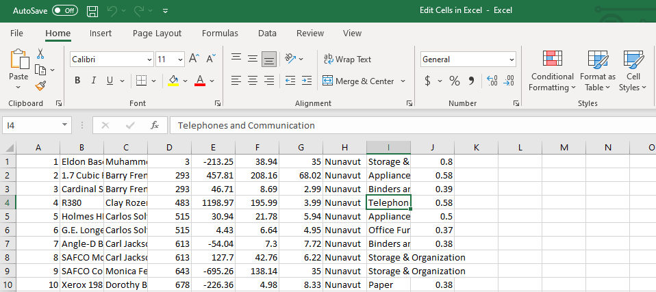
You might not be able to directly edit the contents of a cell by pressing the F2 key.
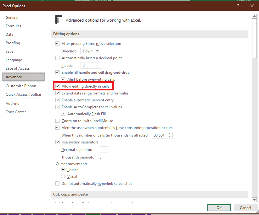
This might be because it has been disabled in Excel. You can easily enable or disable this function by following the steps below:
STEP 1: Click on the File tab
STEP 2: Click Options from the menu on the left side
STEP 3: In the dialog box, click on Advanced from the left panel
STEP 4: Under Editing option, check Allow editing directly in cells. Click OK at the bottom.
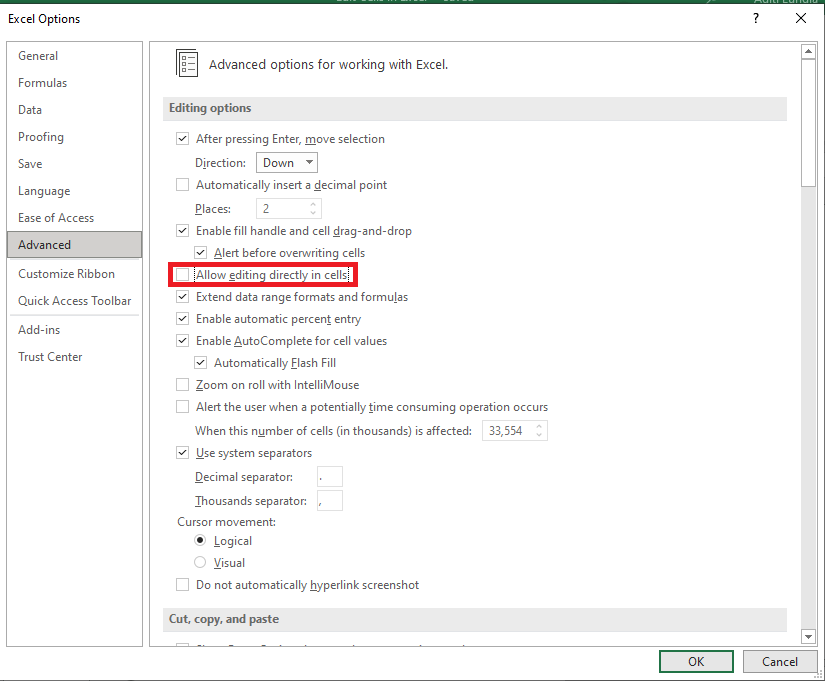
That’s it! Now you can enable the editing cell feature in Excel. To disable Edit mode, clear the Allow editing directly in cells check box.
16. Unable to use the Fill Handle
Excel has many tools that can automate your work and make it much easier and faster. One of these essential tools is the fill handle. It helps fill in a value in the adjoining cells in sequential order of data.
If you are unable to use this feature, it may have been disabled or the filled values are not as per your pattern:
- Fill Handle Excel – not visible
- Not selecting all values
- Auto Fill options
Download workbookFill-handle.xlsx
Example 1: Fill Handle not visible
If you are unable to use this function, you can simply fix it using the steps below:
STEP 1: Select the File tab.
STEP 2: Click Options from the menu on the left side
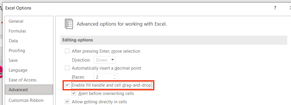
STEP 3: In the Advanced category, under Editing options, select the Enable fill handle and cell drag-and-drop check box.
Once you have enabled this, you can easily use Excel Fill handle feature!
Example 2: Not selecting all values
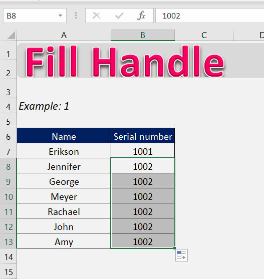
It can even be that you have not selected the entire range that has your sequential values. Just selecting the last cell will fill only that value in the cells where you drag the fill handle in Excel.
For example, if we drag the fill handle after only selecting cell B8, the entire range is filled only with the value “1002”.
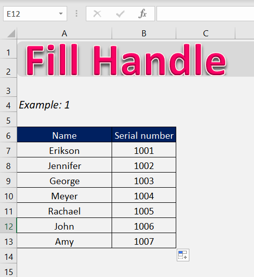
Selecting the entire range and then using the fill handle will fill the new cells in sequential order.
Selecting B7 and B8 will help Excel recognize the pattern and correctly fill the subsequent cells.
Example 3: Auto Fill options
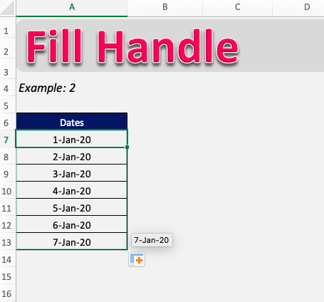
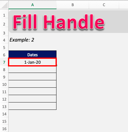
Suppose you have entered the date and you want to use the fill handle to get only weekdays. If you use the fill handle like before, it will just add the next dates in adjacent cells.
You can use the AutoFill option to get dates that are only falling on weekdays!
STEP 1: Select the entered values.
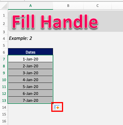
STEP 2: Go to the bottom right of your selection, you can drag the fill handle to fill dates below.
This will fill the dates one after the other!
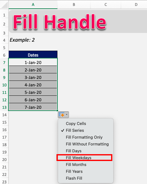
STEP 3: Click on the Fill Handle button at the bottom right.
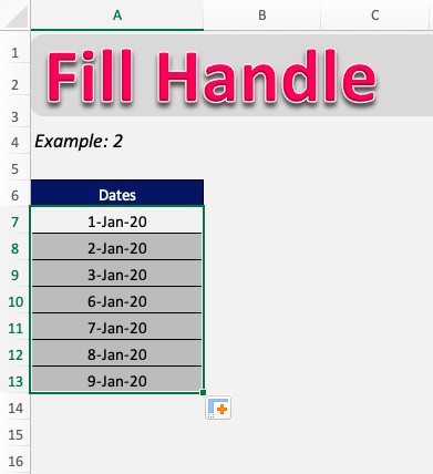
STEP 4: Select Fill Weekdays.
This will just include the weekdays and ignore the weekends like 4-Jan-20 and 5-Jan-20.
You can use other options as well like Fill Formatting only, Fill Months, Flash Fill, etc.
17. Not able to understand the inner workings of a formula
Excel provides a lot of functions at your disposal for efficient working and data management. Formulas can be used widely in Excel to overcome or calculate all sorts of different informational data.
But these formulas can be tough to decipher at first, especially the working of a formula. Here is how you can better understand a formula:
Solution:
When you enter a formula in the cell, you can press Ctrl+A to enter the function arguments window. This shows a detailed explanation of each segment of the formula so that you know which data to feed in which segment and get accurate results.
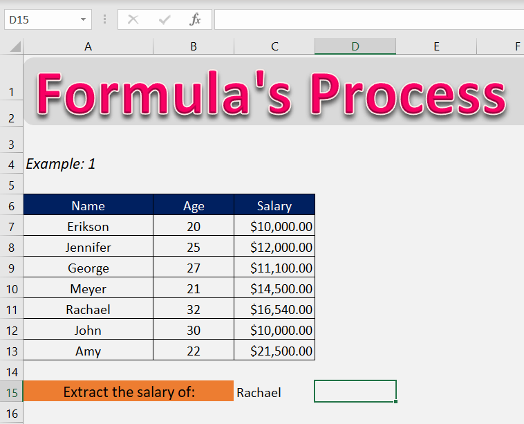
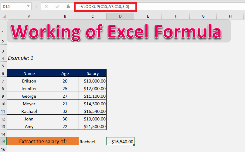
To better understand this, let us take the example using the VLOOKUP formula. Here, we need to extract the salary of Rachael in cell D15.
download excel workbookUnderstand-Excel-Formula.xlsx
Let’s open the arguments wizard for the VLOOKUP formula.
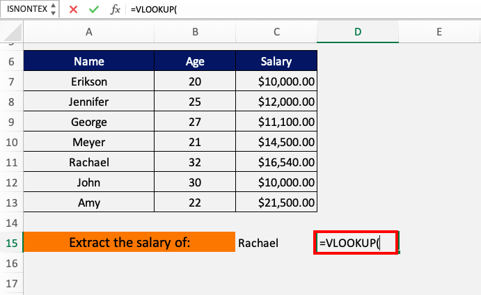
STEP 1: Enter the VLOOKUP function: =VLOOKUP(
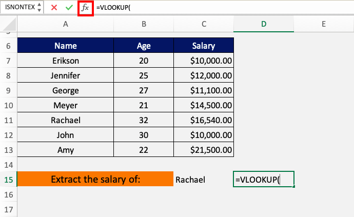
STEP 2: Press Ctrl+A or click on the fx button in the formula bar to open the arguments wizard window.
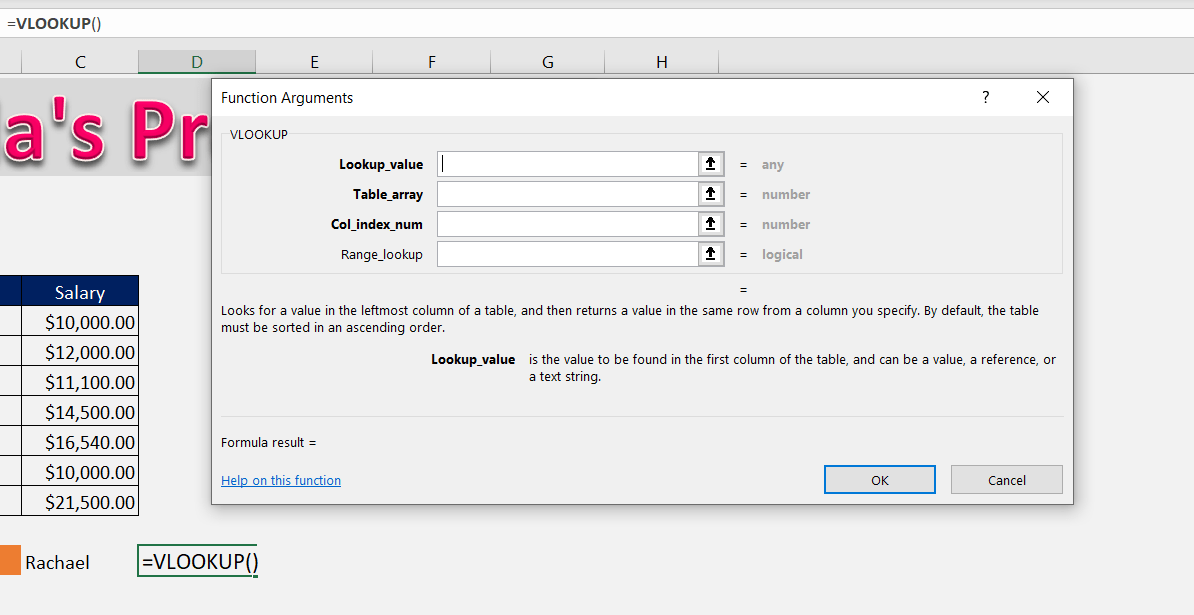
This is how the formula wizard looks like.
It shows all the arguments in sequential order. It then explains the use of the function and the details of the argument selected.
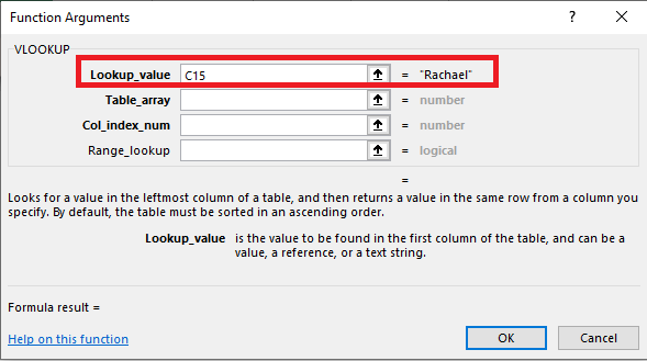
STEP 3: Select the first argument i.e. Lookup_value. Here, cell C15 contains the name, Rachael.
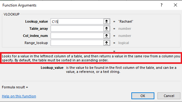
You can also see the description of the first argument is written at the bottom of the dialog box.
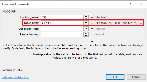
STEP 4: Select the second argument i.e. Table_array and select the table range from where you can search i.e. A7:C13.
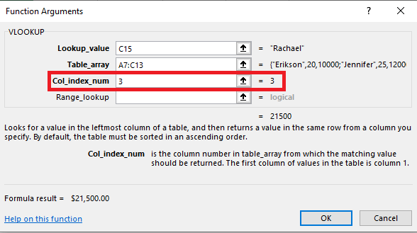
STEP 5: Select the third argument i.e. col_index_num and enter the column number from which to extract the data. In this example, it should be 3.
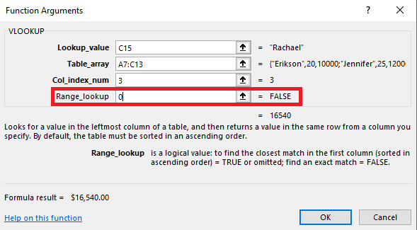
STEP 6: Lastly, select the fourth argument i.e. range_lookup. Since we want an exact match type FALSE or 0.
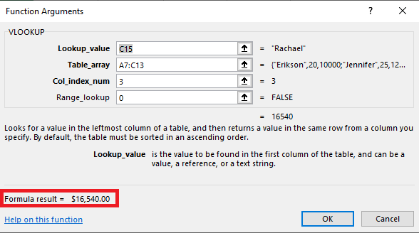
After entering the details, the wizard would look like below. It would even show a preview of the argument values and the answer below it if the inputs were correct.
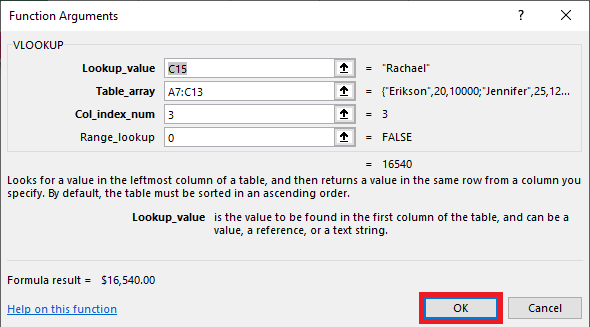
STEP 7: Press OK.
The formula will be entered in cell D15 and it will show the result, i.e., the salary of Rachael – $16,540.
Ctrl+A opens the Function Arguments window immediately after typing the name of the function.
Now that you can easily understand each formula, have fun working on Excel!
18. Cells showing formulas instead of calculated values
While working on an Excel worksheet with a lot of formulas in it, it can become challenging to keep track of all your formulas.
It may happen that the formulas entered in each cell is displayed on the worksheet instead of the value/result.
You can easily reverse this and display the result instead of formula. Let’s see how it can be done!
download excel workbookShowing-Formula.xlsx
Solution:
Ctrl + ` is the shortcut for the formula view, pressing it can change it back to normal view and show your calculated values.
Now you have your cells showing calculated values instead of formulas applied. Try it yourself!
19. Formula does not update when value changes
Excel provides dynamic formulas that update their calculated value as soon as the source data is altered.
An issue faced by people can be that the cells are not updating automatically ,i.e, they are showing the old values even when the dependent cell’s values have been changed. Here is how you fix this issue.
Solution:
The issue that you are facing is most likely caused by an accidental change in the calculation setting from Automatic to Manual. Steps to change this are:
Go to Formula Tab > Calculation Options > Automatic.
Now your formulas will be getting updated which changes in the source data. Now you try it!
20. Formula not working due to text format in cells
Sometimes even when have entered a number in the cell, it is stored as text and thus produce error while computing in Excel.
download excel workbookFormula-not-working.xlsx
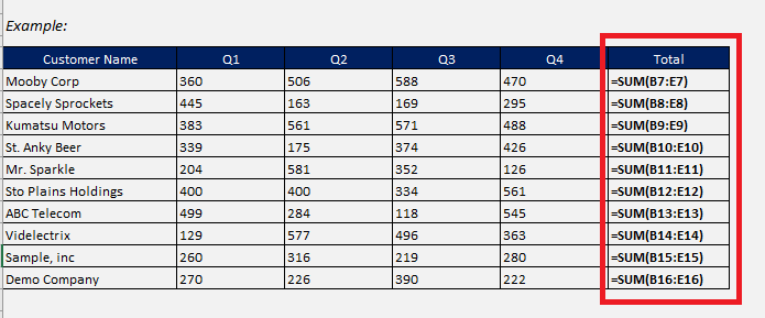
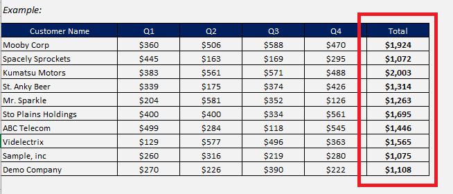
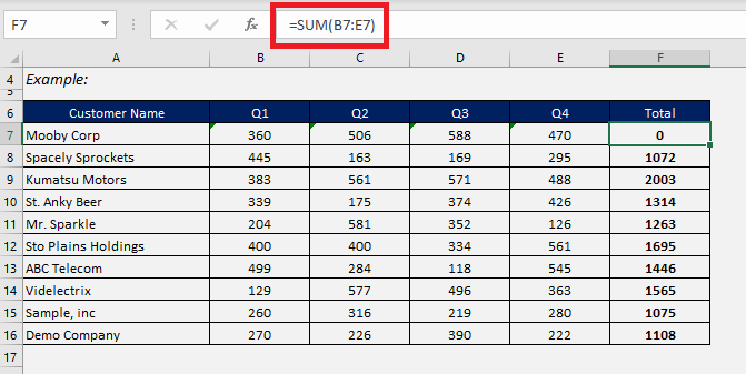
In this example, cell F7 uses sum function to calculate the total amount for all 4 quarters. Even though there are figures in range B7 to E7 the calculated amount in cell F7 is 0.
This is because each of these number are actually stored as text.
Solution:
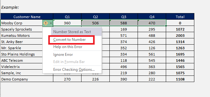
Select the cells that are the source for the formula calculation. Click on the yellow triage icon and select Convert to text.
This will convert the text to number and now the calculated amount will also display the correct value!
It is that simple! Now you try it!
Conclusion
This completes our tutorial on the Top 20 common errors like REF error, NUM error, Excel #### error, etc. that we can encounter while working on Excel.
Now that these common issues are out of your way, we hope that your Excel operations have improved. If you want to continue this journey of improvement, you can further check out our blog as well as our YouTube channel. They offer a ginormous amount of content, a huge library of information provided to you for free.
See you next time!
Make sure to download our FREE PDF on the 333 Excel keyboard Shortcuts here:
John Michaloudis is a former accountant and finance analyst at General Electric, a Microsoft MVP since 2020, an Amazon #1 bestselling author of 4 Microsoft Excel books and teacher of Microsoft Excel & Office over at his flagship Academy Online Course.

