I have shown my Free Pivot Table webinar to over 40,000 people over the last couple of years and I continually get the same questions from my webinar attendees regarding the little issues they have when using a Pivot Table.
I want to put Excel Pivot Table issues to bed so you can go out and use a Pivot Table to analyze lots of data and create interactive Dashboards with key business metrics, rather than worry about these small nuances.
So in this quick tutorial I will show you how to:
Table of Contents
Want to know how to create Excel Dashboards?
#1 SUM RATHER THAN COUNT
The no1 complaint that I get is “Why do my values show as a Count of rather than a Sumof ?”
Well, there are three reasons why Pivot Table not counting correctly:
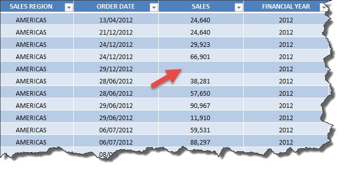
1. There are blank cells in your values column within your data set; or
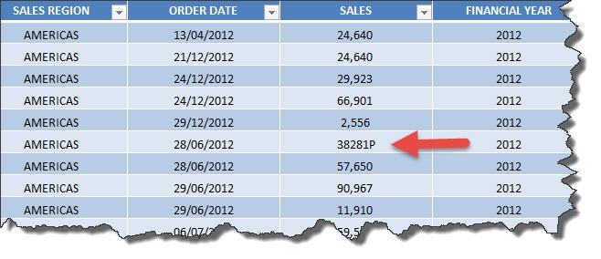
2.There are “text” cells in your values column within your data set; or
3. A Values field is Grouped within your Pivot Table.
1. BLANK CELL(S):
So if you have at least one blank cell in a Values column, Excel automatically thinks that the whole column is text-based. Pretty stupid but that’s the way it thinks.
2. TEXT CELL(S):
Also if you have a cell that is formatted as Text within your Values column, then it will also cause it to Count rather than Sum.
This usually happens when you download data from your ERP or external system and it throws in numbers that are formatted as text e.g. 382821P
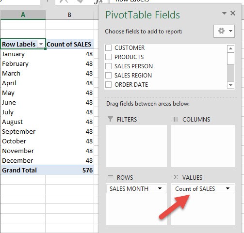
Pivot Table not showing correct data and you will get the annoying Count of Sales below:
Have a look at the following tutorials that show you how to locate blank cells.
Find Blank Cells In Excel With A Color
EXCEL FIX:
STEP 1: You will need to enter a value or a zero within this blank or text formatted cell(s)
STEP 2: Go over to your Pivot Table, click on the Count of…. and drag it out of the Values area
STEP 3: Refresh your Pivot Table
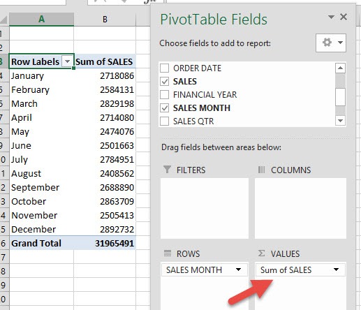
STEP 4: Drop in the Values field (SALES) in the Values area once again
3. GROUPED VALUES:
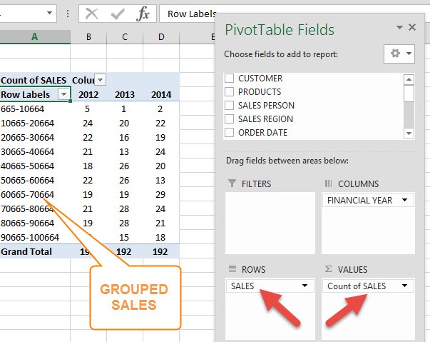
Let’s say that you put a Values field (e.g. Sales) in the Row/Column Labels and then you Group it.
When you drop in the same Values field in the Values area, you will also get a Count of…
EXCEL FIX:
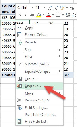
STEP 1: Right Click on the Grouped values in the Pivot Table and choose Ungroup:
STEP 2: Drag the Count of SALES out of the Values area and let go to remove it
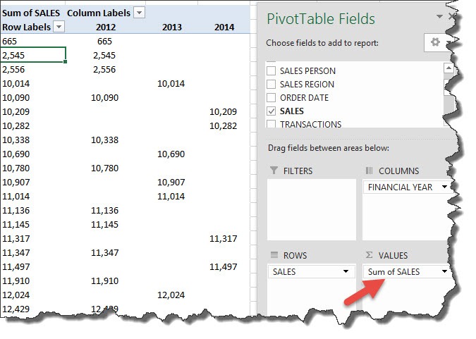
STEP 3: Drop in the SALES field in the Values area once again
It will now show a Sum of SALES!
N.B. Sometimes you will need to locate the Pivot Table that has the Grouped values. The SALES field may not be evident that it is Grouped, especially if it is not selected in the Row/Column labels.
You may need to drag and drop this field from the PivotTable Fields and into the Row/Column Labels area to confirm that it is Grouped.
#2 FIXED NUMBER FORMATS
The no.2 request that I get is “Is there a way to have predetermined value formatting in the Pivot Table so we do not have to always format the values each time we create a Pivot Table?”
Well YES there is…sort of!
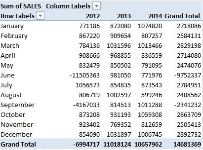
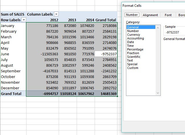
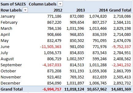
When you create a new Pivot Table it will always format the cells without any commas or decimal points, which is very hard to read, especially if you have positive and negative numbers that go into the millions.
Here I show you how to overcome Pivot Table Issues:
EXCEL FIX:
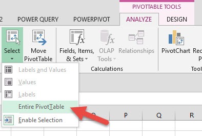
STEP 1: Click inside your Pivot Table and go to PivotTAble Tools > Analyze/Options > Select > Entire Pivot Table
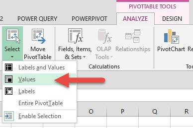
STEP 2: Go back into PivotTable Tools > Analyze/Options > Select and this time choose the Values option
STEP 3: Press CTRL+1 which will bring up the Format Cells dialogue box
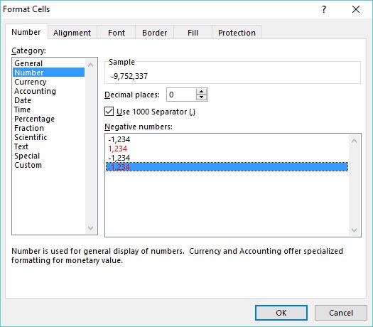
STEP 4: Choose the Number category and select the format that you want, then press OK:
Your Pivot Table is now formatted!
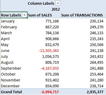
You can now drop in more Values fields (like TRANSACTIONS numbers) in the Values area and it will also keep the same formatting:
You can also copy and paste this Pivot Table and rearrange it and the formatting will still be kept!
Cool hey.
#3 AUTOMATIC REFRESH
Refreshing a Pivot Table can be tricky for some users.
People forget that each time your data source gets updated that you will also need to Refresh your Pivot Table in order for it to get updated and reflect the changes.
A lot of people ask if there is a way to automatically Refresh a Pivot Table, which I totally get.
Here I show you a couple of ways that you can fix these pivot table problems.
1. REFRESH PIVOT TABLE UPON OPENING:
This is a great feature and one that most people don’t know about.
It allows you to Refresh your Pivot Tables as soon as you open up your Excel workbook.
This is great if your Pivot Table’s data is linked to another workbook that gets updates by your colleagues and you only get to see the Pivot Table report. Otherwise, they may think that the Pivot Table not working.
EXCEL FIX:
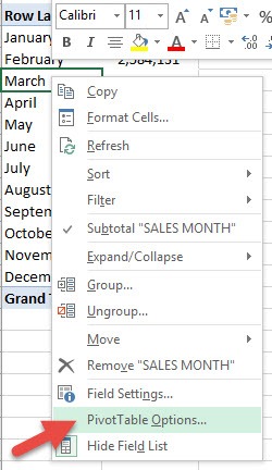
STEP 1: Right Click in your Pivot Table and choose Pivot Table Options:
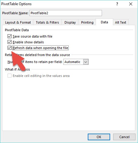
STEP 2: Select the Data tab and check the “Refresh data when opening the file” checkbox and OK
Now each morning that you open up your Excel workbook, you can be sure that the Pivot Table is refreshed!
2. AUTOMATIC REFRESH EVERY X MINUTES:
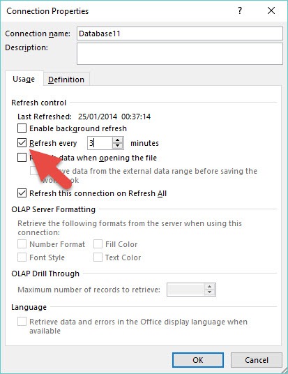
If you have your data set linked in an external data source, you can auto-refresh every x minutes.
Your data can be stored in an external data source such as Access, a Website, SQL Server, Azure Marketplace etc
EXCEL FIX:
STEP 1: If your data is stored externally, you will need to click in your Pivot Table and go to Properties (this will only be enabled for selection if you have an external data source)
STEP 2: This will open up the Connection Properties and you will need to select the Refresh every checkbox and manually set the time & press OK.
You can now sit back and enjoy a cup of coffee whilst your Pivot Table gets updated every few minutes:)
Further Learning:
- Unleashing the Power of Pivot Tables in Excel: A Practical Guide
- Excel Pivot Cache Explained
- Show/Hide Field Headers in Excel Pivot Tables
I hope that you enjoyed this article and can now get over these little nuances and spend your valuable time where it is needed, analyzing your data & making insightful reports with your Pivot Table 🙂
Feel free to comment below and let me know what Pivot Table issues you have and I will resolve them for you.
Make sure to download our FREE PDF on the 333 Excel keyboard Shortcuts here:
John Michaloudis is a former accountant and finance analyst at General Electric, a Microsoft MVP since 2020, an Amazon #1 bestselling author of 4 Microsoft Excel books and teacher of Microsoft Excel & Office over at his flagship Academy Online Course.
