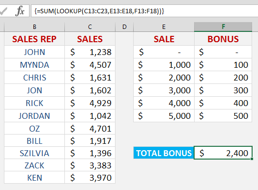
The LOOKUP function has three arguments, it is a like a simplified VLOOKUP function:
What does it do?
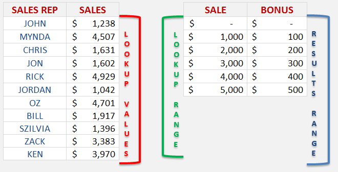
It looks up a value (lookup_value) in one range (lookup_vector) and returns a value from the same position in a second range (result_vector)
Formula breakdown:
=LOOKUP(lookup_value, lookup_vector, result_vector)
What it means:
=LOOKUP(The value that you want to lookup, Range that contains the values to be lookup up, Range that contains the values to be returned)
** Note that the LOOKUP function uses the Approximate Match argument automatically (TRUE argument in a VLOOKUP), so therefore the result_vector has to be sorted in ascending order **
Read this blog that explains the VLOOKUP using the Approximate or TRUE argument
Say that you want to calculate the Total Bonuses due to the Sales Reps, you can do that using the SUM(LOOKUP()) formula and then pressing CTRL+SHIFT+ENTER to turn it into an Array formula.
You will need to have your data set up into three separate columns, one for the Lookup Values (Sales made by the Sales Rep), another for the Lookup Range (Sales bonus threshold) and the last one for the Results Range (Bonus payable in ascending order)
Download excel workbookArray-Sales-Bonuses.xlsx
STEP 1: Enter the SUM function =SUM(
STEP 2: Nest the LOOKUP function =SUM(LOOKUP(
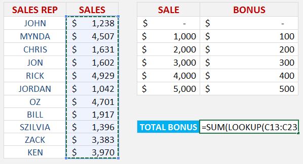
STEP 3: Select the Lookup Values in the Sales Rep Sales column:
=SUM(LOOKUP(C13:C23,
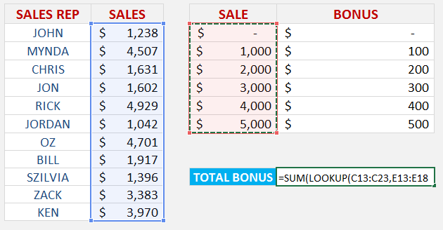
STEP 4: Select the Lookup Range in the Sale bonus threshold column:
=SUM(LOOKUP(C13:C23,E13:E18,
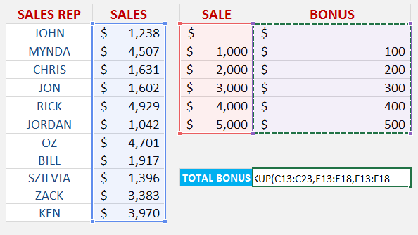
STEP 5: Select the Results Range in the Bonus payable column:
=SUM(LOOKUP(C13:C23,E13:E18,F13:F18
STEP 6: Instead of pressing ENTER to evaluate the formula, you need to press CTRL+SHIFT+ENTER to turn the formula into an Array Formula which will look like this:
{=SUM(LOOKUP(C13:C23,E13:E18,F13:F18))}
STEP 7: By pressing F9 on the selected formula array will give you the resulting array of numbers that get summed up (press CTRL+Z to get out of this mode when you are done checking the formula results):
John Michaloudis is a former accountant and finance analyst at General Electric, a Microsoft MVP since 2020, an Amazon #1 bestselling author of 4 Microsoft Excel books and teacher of Microsoft Excel & Office over at his flagship Academy Online Course.
