Power Query lets you perform a series of steps to transform your Excel data. One of the steps it allows you to take is to transpose data very easily.
Transposing a data table is basically rotating your data from rows to columns, or from columns to rows. To further explain this concept, screenshots are provided below.
Download excel workbookTranspose.xlsx
Let’s go through the steps in detail:
STEP 1: Select your data and turn it into an Excel Table by pressing the shortcut Ctrl + T or by going to Insert > Table
STEP 2: Go to Data > Get & Transform > From Table (Excel 2016) or Power Query > Excel Data > From Table (Excel 2013 & 2010)
Excel 2016:
Excel 2013 & 2010:
STEP 3: This will open up the Power Query Editor.
We want to rotate this data from rows to columns.
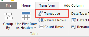
STEP 4: Within here you need to select Transform > Transpose
STEP 5: Now you will see your changes take place.
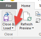
STEP 6: Click Close & Load from the Home tab and this will open up a brand new worksheet in your Excel workbook with the transposed data.
You now have your new transposed table.
HELPFUL RESOURCE:
Bryan
Bryan is a best-selling book author of the 101 Excel Series paperback books.


