There are various lookup functions that bring back values from a range of data like the VLOOKUP, INDEX, INDEX-MATCH and OFFSET functions, just to name a few.
There is another lookup formula that you can use that will return the intersection of two Named Ranges!
This is done by using the SUM formula and entering a Named Range for the 1st argument and then pressing the SPACE BAR on your keyboard (thus activating the intersection) and entering a 2nd Named Range.
This combination will look at the intersection of the 1st Named Range and the 2nd Named Range and return that cell’s value. I show you how below…
Download excel workbookSum-Interesction.xlsx
STEP 1: Highlight your data which has to have Column headings and Row headings, just like the table below:
STEP 2: Go to the ribbon menu and select Formulas > Create from Selection
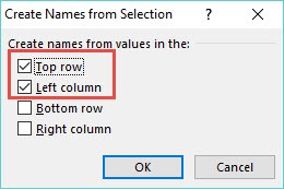
STEP 3: This will bring up the Create Names from Selection dialogue box. Choose the Top Row and Left Column boxes, as this is where your headings are located and press OK:
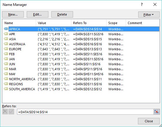
STEP 4: In the ribbon menu, go to Formulas > Name Manager to see the Named Ranges that were created in Step 3
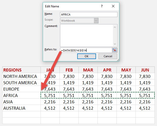
You can double click on a Named Range and click on the Refers to area to see the range (press ESC to get out of this screen):
STEP 5: Enter the SUM function and in the first argument type in the 1st Named Range:
=SUM(EUROPE
STEP 6: Enter a SPACE after the 1st argument. Now type in the 2nd Named Range:
=SUM(EUROPE MAR)
This will return the intersection of the 1st and 2nd Named Ranges:
You can even make this formula interactive by inserting a drop down menu (data validation) for the Months and the Regions!
John Michaloudis is a former accountant and finance analyst at General Electric, a Microsoft MVP since 2020, an Amazon #1 bestselling author of 4 Microsoft Excel books and teacher of Microsoft Excel & Office over at his flagship Academy Online Course.


