Excel Slicer was first introduced in Pivot Tables in Excel 2010 for Windows and Excel 2016 for Mac.
Pivot Table Slicers are a visual filter in the form of an interactive button. There are several cool things that you can do with Pivot Table Slicer, like customize them, filter them, connect them to multiple Pivot Tables plus much more!
Learn How to Create Interactive employee photos with Excel Slicer!
*** Watch our video and step by step guide below with a free downloadable Excel workbook to practice ***
Topic 2: Different Ways to Filter an Excel Slicer
Topic 3: Add Columns to Slicer Buttons
Topic 4: Slicer Styles & Settings
Topic 5: Connect Slicers to Multiple Excel Pivot Tables
Topic 6: Lock The Excel Pivot Table But NOT The Slicer!
BONUS: Free Excel Pivot Table Webinar Training!
1. Insert a Slicer
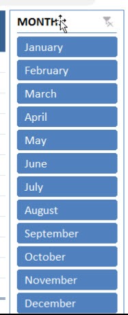
Excel Slicer is visual filter or interactive button that allow you to see what items have been chosen within a Pivot Table.
They are a new feature from Excel 2010 onward and Mac for Excel 2016 and a must for anyone wanting to wow their boss by adding interactivity in their reports! I show you How to Use Slicer in Excel below:
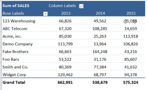
STEP 1: Select your Pivot Table by clicking anywhere inside it.
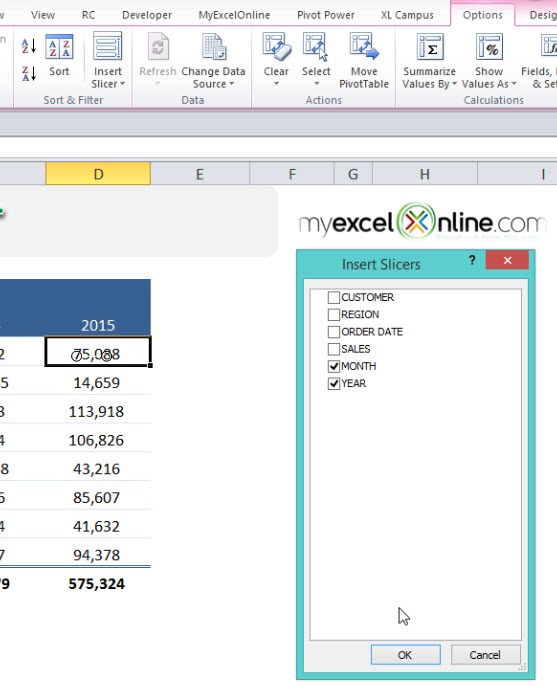
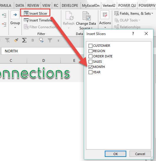
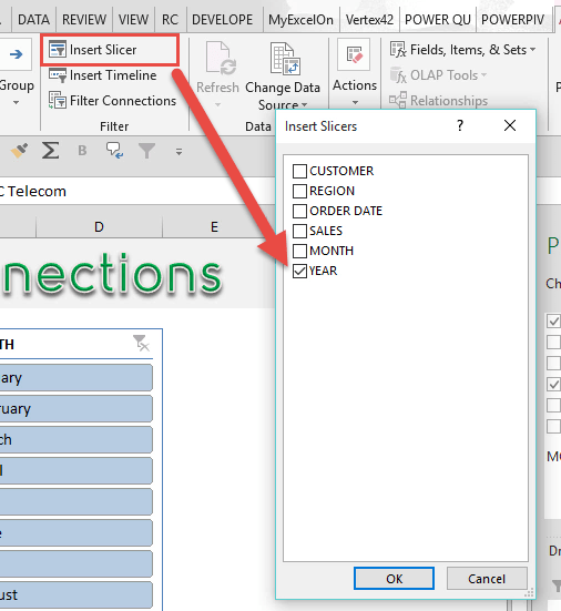
STEP 2: Go to Options(Excel 2010)/Analyze(Excel 2013&2016) > Insert Slicer
Select the Month and Year Fields.
Click OK.
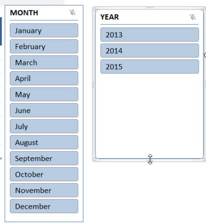
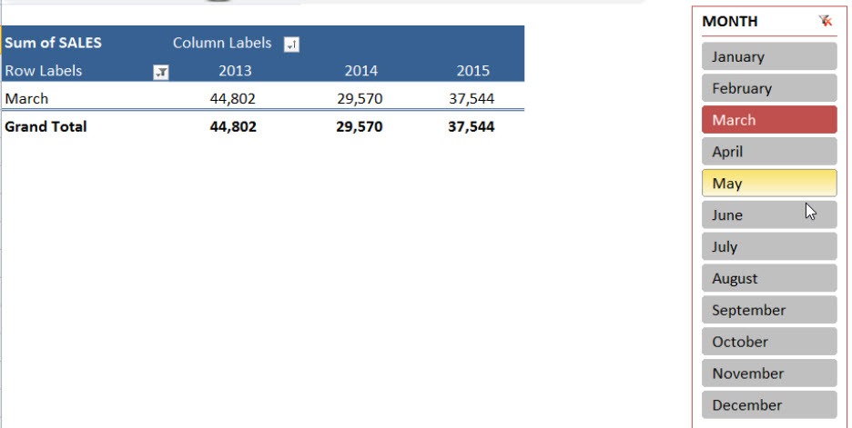
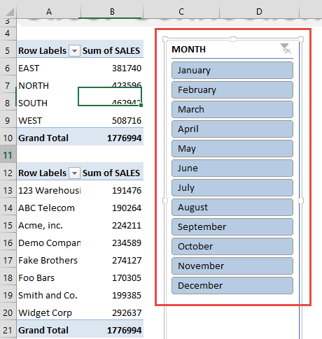
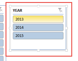
Your slicer is now ready! Go crazy clicking, slicing and dicing your data!
TIP: Hold down the CTRL key to select multiple items in your Slicer.
2. Different Ways to Filter an Excel Slicer
Excel Slicers are the best thing since sliced bread!
They are a new feature from Excel 2010 onward and Mac for Excel 2016 and are visual buttons that show you what items have been filtered or selected in a Pivot Table.
There are several ways that you can filter an Excel Slicer.
Try it now by downloading this free workbook:
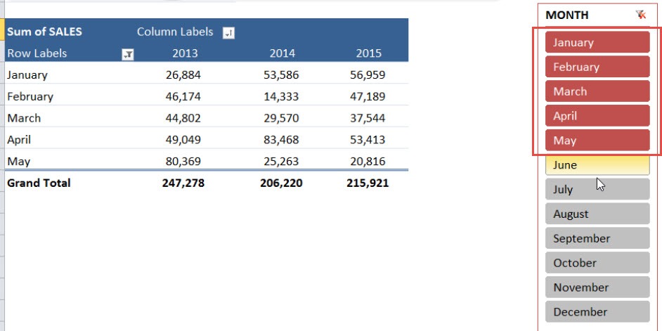
LEFT MOUSE CLICK: You can select items from the Slicer by using your left mouse button;
DRAG LEFT MOUSE BUTTON: You can select an array of items by clicking the left mouse button and doing a dragging motion downwards/upwards within the Slicer;
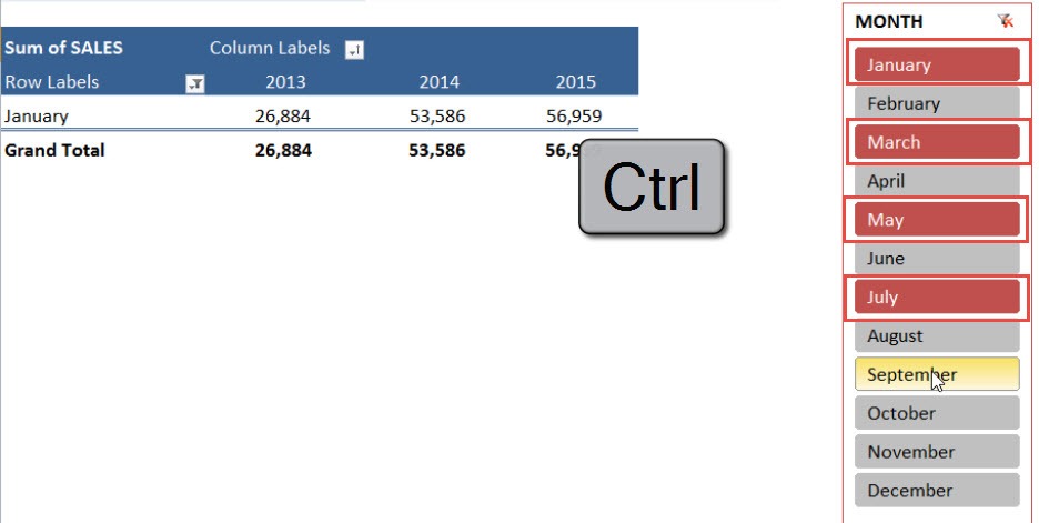
CTRL KEYBOARD: You can select multiple items by holding down the CTRL key on your keyboard;
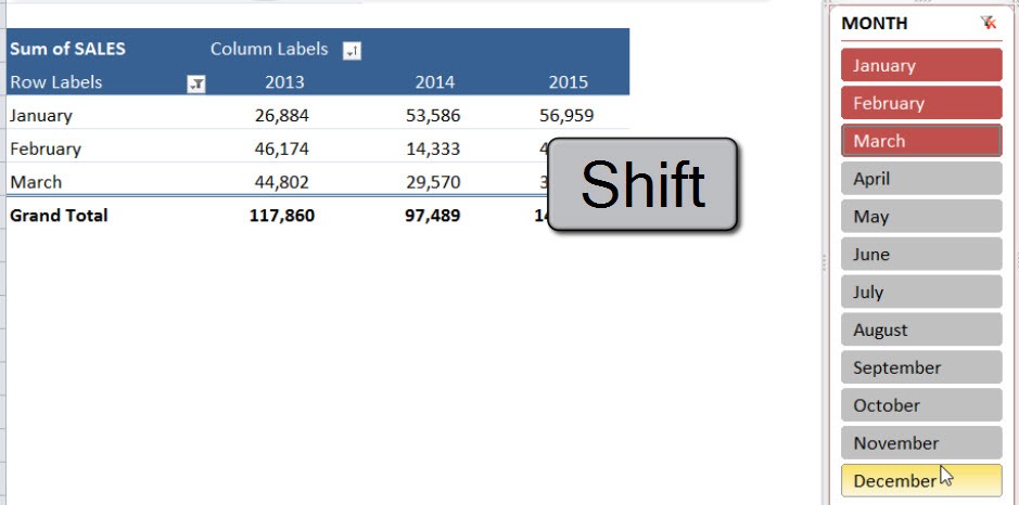
SHIFT KEYBOARD: You can select a range of items by holding down the SHIFT key on your keyboard!
3. Add Columns to Slicer Buttons
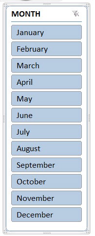
When you insert an Excel Slicer with your Pivot Table it defaults to one column, showing all your items in a vertical layout.
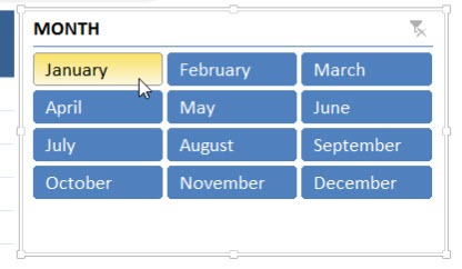
Say that your Slicer is showing months from January to December, you can change the layout of the buttons to show in 3 separate columns, turning it into a “Quarterly View”.
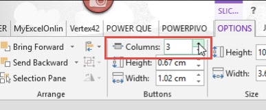
To do this you need to click on your Slicer and go to Slicer Tools > Options > Buttons > Columns. You can then use the scroll bar to increase and decrease the columns or manually type in the number of columns to show your Slicer.
STEP 1: Select your Slicer.
STEP 2: Go to Slicer Tools > Options > Buttons > Columns
Select Columns to 3.
Your slicer now has a 3-column layout!
4. Slicer Styles & Settings
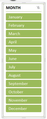
There are several different Slicer Styles available when you click on an Excel Slicer. It is located in the Slicer Tools tab in the Ribbon under Options > Slicer Styles. You can also add columns to a Slicer and you can find more Slicer options by Right Clicking in a Slicer.
STEP 1: Select your Slicer.
STEP 2: Go to Slicer Tools > Options > Slicer Styles
Select a style you prefer.
Your slicer now has a different style!
5. Connect Slicers to Multiple Excel Pivot Tables
Normally when you insert an Excel Slicer it is only connected to the Pivot Table that you are inserting it from.
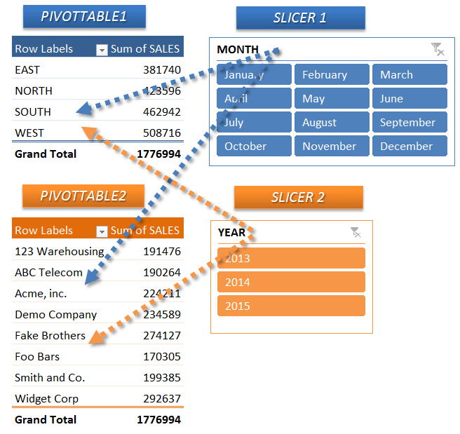
What about if you had multiple Pivot Tables from the same data set and wanted to connect a Slicer to all of the Pivot Tables, so when you press a button all the Pivot Tables change?
Well this is possible with the Report Connections (Excel 2013 & 2016) / PivotTable Connections (Excel 2010) option within the Slicer. This is how it is achieved:
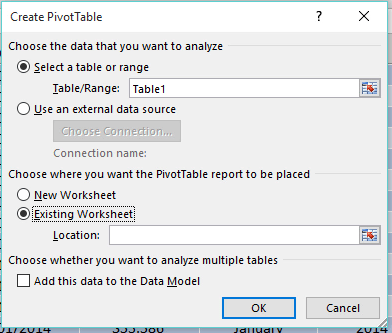
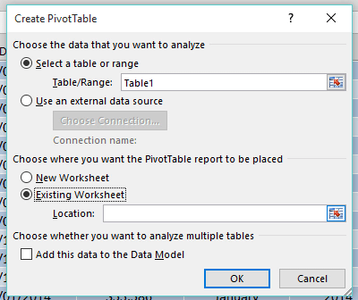
STEP 1: Create 2 Pivot Tables by clicking in your data set and selecting Insert > Pivot Table > New Worksheet/Existing Worksheet
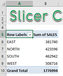
Setup Pivot Table #1:
ROWS: Region
VALUES: Sum of Sales
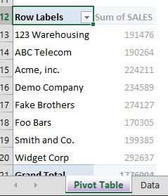
Setup Pivot Table #2:
ROWS: Customer
VALUES: Sum of Sales
STEP 2: Click in Pivot Table #1 and insert a MONTH Slicer by going to PivotTable Tools > Analyze/Options > Insert Slicer > Month > OK
STEP 3: Click in Pivot Table #2 and insert a YEAR Slicer by going to PivotTable Tools > Analyze/Options > Insert Slicer > Year > OK
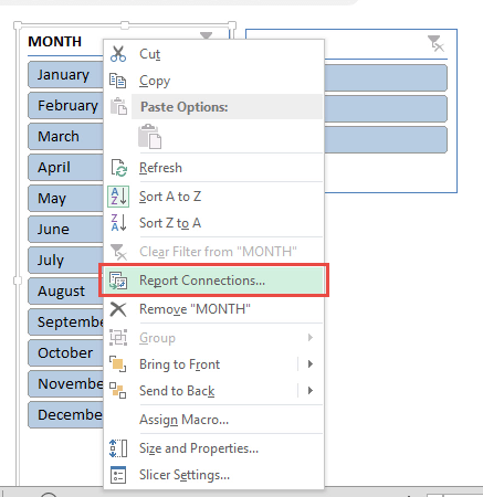
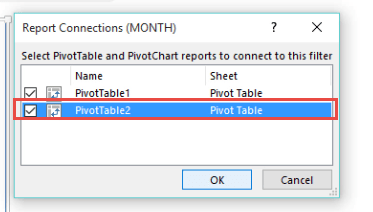
STEP 4: Right Click on Slicer #1 and go to Report Connections(Excel 2013 & 2016)/PivotTable Connections (Excel 2010) > “check” the PivotTable2 box and press OK
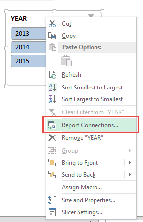
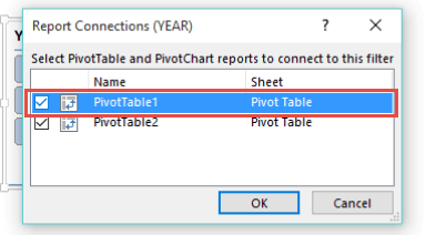
STEP 5: Right Click on Slicer #2 and go to Report Connections(Excel 2013)/PivotTable Connections (Excel 2010) > “check” the PivotTable1 box and press OK
Now as you select each Slicer’s items, both Pivot Tables will change!
Have a look at the following image and the tutorial below that to see how this is achieved using Excel 2013:
6. Lock The Excel Pivot Table But NOT The Slicer!
Sometimes when you are sharing an Excel Pivot Table with your colleagues you do not want the other user(s) to mess with your Pivot Table layout and format.
What you can do is lock the Pivot Table and only allow the user(s) to select the Slicers, making your report interactive and secure from Excel novices like your boss 🙂
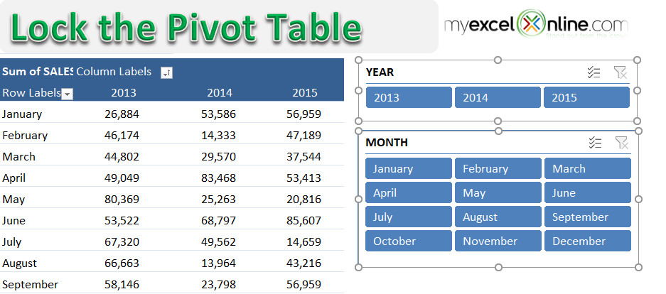
Here is how you can lock the Pivot Table but not the Slicers:
Download locked excel workbookLock-the-workbook-Locked.xlsx
(Password to unlock: myexcelonline)
STEP 1: Click on a Slicer, hold the CTRL key and select the other Slicers
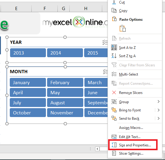
STEP 2: Right-click on a Slicer and select Size & Properties
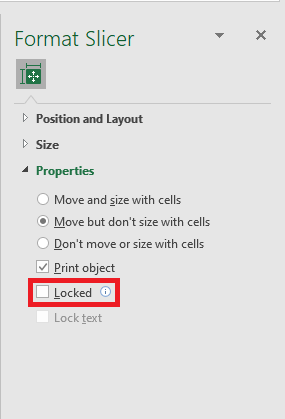
STEP 3: Under Properties, “uncheck” the Locked box and press Close
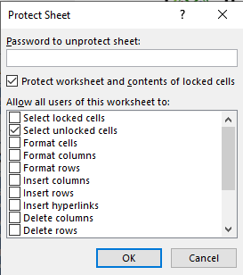
STEP 4: Go to the ribbon menu and select Review > Protect Sheet
STEP 5: “Uncheck” the Select Locked Cells and “Check” the Select Unlocked Cells & Use Pivot Table Reports
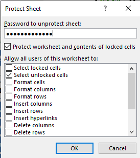
STEP 6: Enter a password (optional) and press OK
Further Learning:
- Use One Slicer for Two Excel Pivot Tables
- The Ultimate Guide to Excel Pivot Table Slicers
- Connect Slicers to Multiple Excel Pivot Tables
Free Excel Pivot Table Webinar Training!
If you liked all the above cool Slicer tips, then you will love my free Excel Pivot Table webinar where I show you more cool Slicer tricks, as well as various Pivot Table features like: Grouping, Year To Data Analysis, Variance Analysis and I will also show you how to create an interactive Excel Dashboard!
Click below to join for free and learn all these cool Pivot Table features that will make you stand out from the crowd…
Bryan
Bryan is a best-selling book author of the 101 Excel Series paperback books.

