Microsoft Excel‘s Split Screen feature revolutionizes how we handle large spreadsheets by allowing simultaneous viewing and editing of different sections. This function is crucial for maintaining focus on various data points without losing your place, enhancing both accuracy and efficiency in your workflow.
Key Takeaways
- Enhanced Productivity: Split Screen enables you to view multiple parts of a worksheet at once, significantly reducing the need for constant scrolling and tab switching.
- Ease of Comparison: This feature simplifies the comparison of disparate data sets by keeping them visible simultaneously, which helps in recognizing trends and discrepancies quickly.
- Flexible Viewing Options: Excel allows vertical, horizontal, or combined splits, catering to different types of data review and analysis needs.
- Independent Scrolling: Each pane operates independently, allowing for focused examination of specific data while referencing other parts of the spreadsheet.
Table of Contents
Optimizing Your Excel Workflow with Split Screen
What Is Split Screen in Excel?
Imagine working on a large spreadsheet and needing to compare your monthly sales from two different quarters that are several rows apart. Without split screen, you’d scroll back and forth, losing track and possibly missing out on critical insights.
Split screen in Excel is a lifesaver here, as it allows you to divide your workbook into separate panes that can independently scroll through different areas of your data. You can view and edit multiple sections of your spreadsheet simultaneously, ensuring no detail slips through the cracks.
The Advantages of Using Split Screen for Data Analysis
Using split screen in Excel isn’t just a nifty trick; it’s a strategic move that could make a significant impact on your data analysis process. First off, it dramatically improves your productivity by allowing you to work on different parts of your worksheet without switching tabs or losing your place. Imagine being able to keep an eye on your summary totals while entering data several rows down—all at the same time.
Plus, it makes comparisons a breeze; you can easily cross-reference information without the tedious scrolling back and forth, saving you time and reducing errors. With focused analysis, you’ll spot patterns, trends, and discrepancies quicker, as important data can stay in view while you investigate other sections.
For those navigating through large datasets, split screens keep headers and labels visible, maintaining your bearings and allowing for efficient, smoother navigation.
Getting Started with Excel Split Screen
How to Activate Split Screen Feature
Activating the split screen feature in Excel is a straightforward task that will open up a world of efficiency for you. To get started, follow these simple steps:
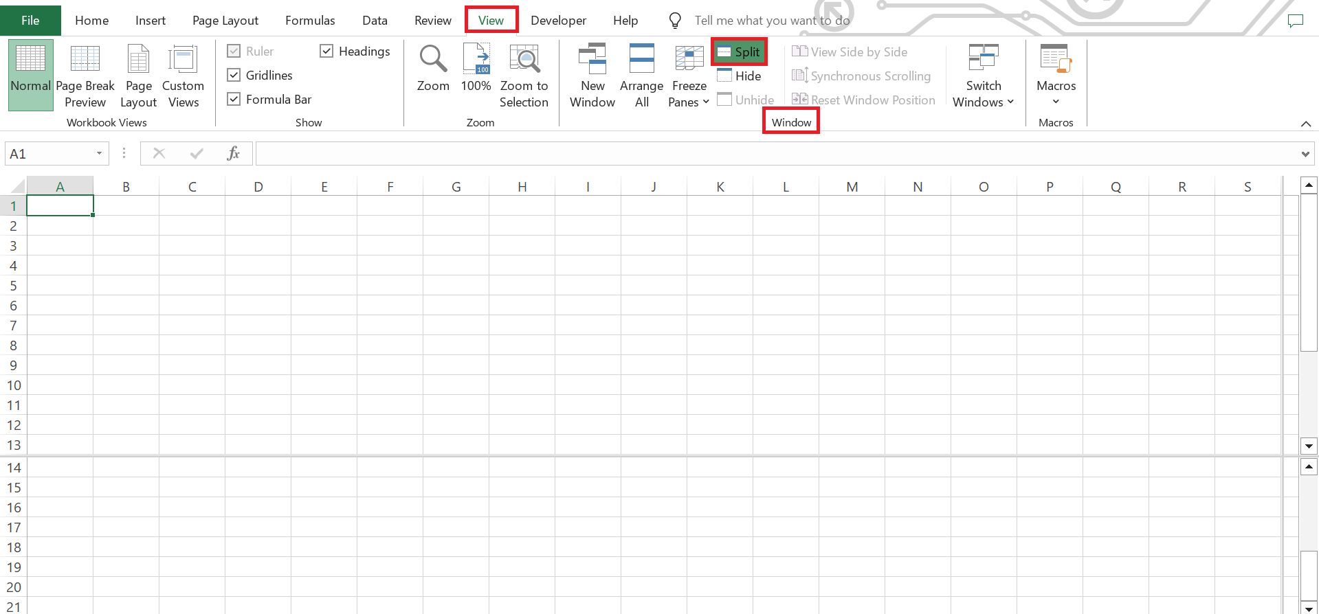
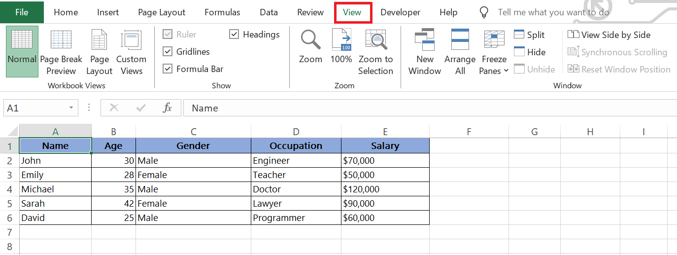
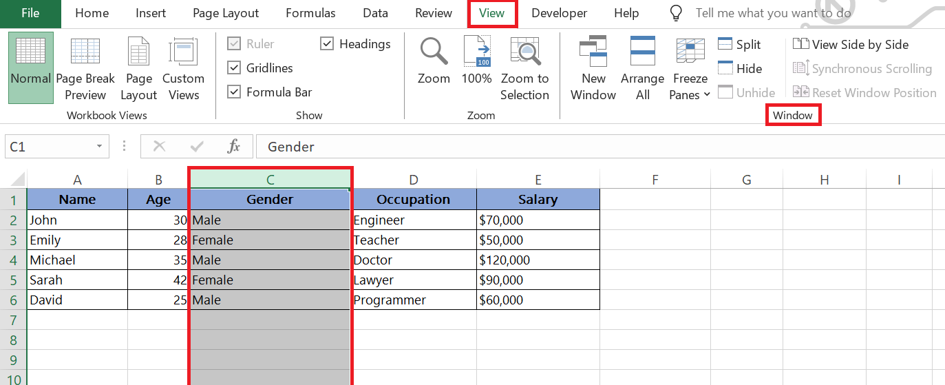
STEP 1: Launch your Excel workbook and click on the “View” tab.
STEP 2: In the “Window” group, look for the “Split” option.
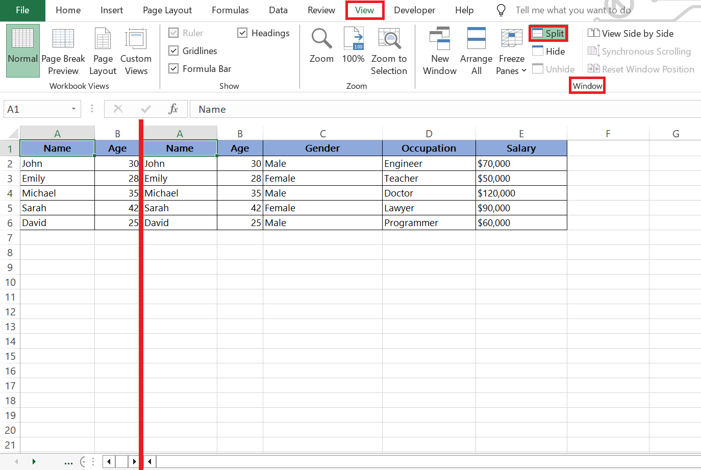
STEP 3: Click on the “Split” button and voilà! Your screen will divide into two or four panes depending on where you’ve positioned your cursor.
What’s excellent here is the flexibility. You decide whether to split your window vertically, horizontally, or both ways by placing the cursor accordingly before clicking “Split.” If you only want to compare rows, click on a cell in the topmost row you need and hit “Split.” For columns, do the same along the leftmost column.
Advanced Split Screen Techniques
Splitting the Screen Both Horizontally and Vertically
Are you juggling multiple data sets that require constant back-and-forth? Splitting your Excel screen both horizontally and vertically allows you to see different sections of your worksheet simultaneously, without endlessly scrolling. Here’s how you can do just that:
To create a horizontal split:
STEP 1: Go to the “View” tab and in the “Window” group,
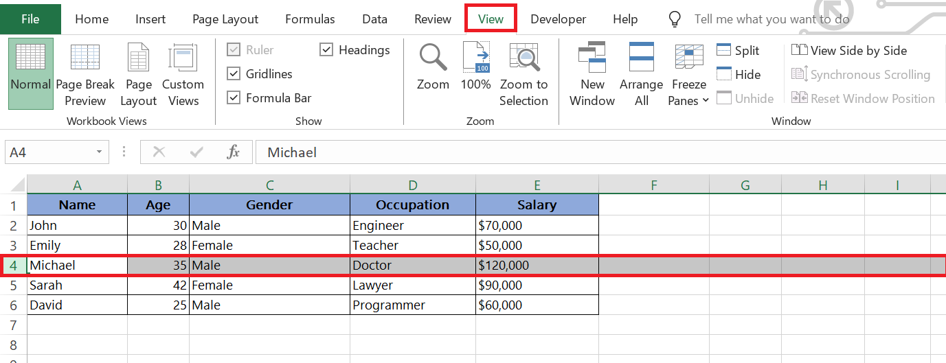
STEP 2: Select the row below where you want the split to occur.
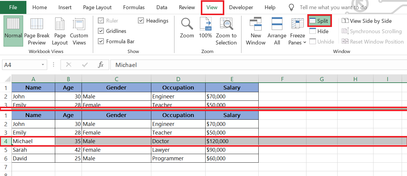
STEP 3: Click on “Split.” This divides the data from the selected row and two screens are created which help in analyzing each variable side by side and make a comparative analysis.
For a vertical split:
STEP 1: Go to the “View” tab and in the “Window” group,
STEP 2: Select the column beside where you want the split to occur
STEP 3: Click on “Split.” This divides the data from the selected column into two screens which helps in making comparison.
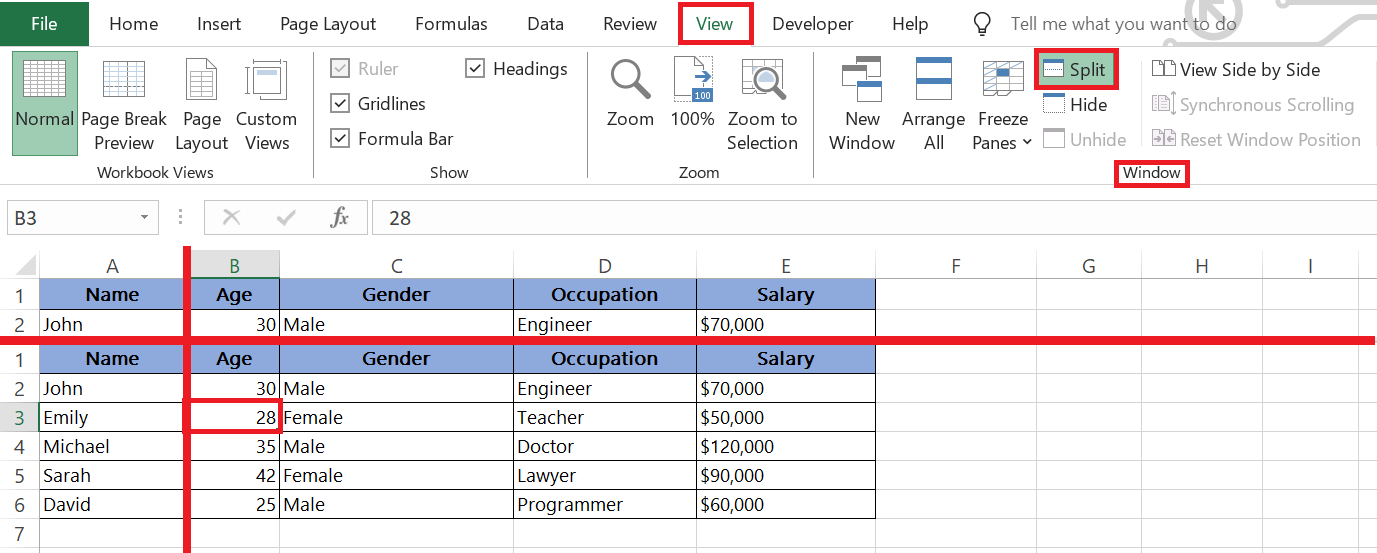
To see the magic of both:
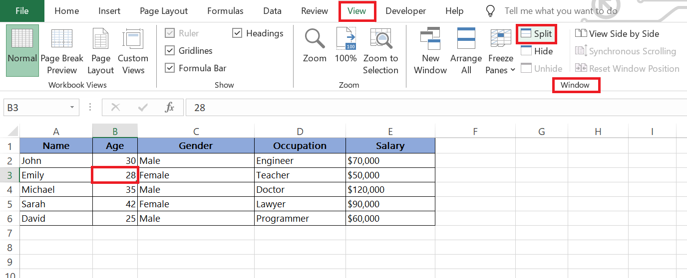
STEP 1: Click on a cell that is not in the first column or row.
STEP 2: Choose “Split” from the “View” tab as before.
Don’t worry if you need to adjust after applying the split—you can click and drag the split lines to fine-tune the size of each pane until it fits your needs just right.
Mastering Navigation within the Split Screen
How to Scroll Harmoniously in a Split View
Navigating a split view in Excel can feel a bit tricky at first, but with a few tips, you’ll be scrolling through your data harmoniously in no time. Each pane in the split screen operates independently – that means scrolling in one pane doesn’t affect the others. This is perfect for comparing distant sections of your worksheet without losing your place.
However, if you need to scroll through the split panes simultaneously, that’s where synchronous scrolling comes into play. You can turn it on by going to the “View” tab and clicking “Synchronous Scrolling” in the “Window” group. Now, when you scroll in one pane, the others follow suit—a real magic trick when lining up data for side-by-side analysis.
Remember to adjust synchronous scrolling to match your task at hand, as it works best when the rows or columns correspond across panes.
Practical Applications of Excel Split Screen
Comparative Analysis Made Easier with Split View
Split view is a silver bullet when it comes to conducting comparative analysis in Excel. Imagine needing to compare annual sales figures with monthly expenses, or having to align different datasets to draw parallels. Split view allows you to have these datasets in parallel sightlines, reducing the risk of eye strain and misinterpretation that often comes from flipping back and forth between tabs or scrolling cumbersome distances.
By placing two sets of data side by side or one above the other, you enable a clear, focused comparison. You can also sort and filter data in one pane without affecting the content in another, which is particularly handy during an in-depth analysis.
Whether you’re tracking performance metrics, crunching financials, or reviewing inventory lists, the split view lets you juxtapose variables effortlessly and draw out the relationships between disparate yet related data chunks.
Multi-Tasking on Different Worksheets Simultaneously
Excel’s ability to display different worksheets from the same workbook at the same time is a multitasker’s dream. By harnessing the New Window feature, you can view and work on two or more sheets side-by-side, making drag-and-drop between worksheets a piece of cake.
For instance, if you’re crafting a budget and need data from last year’s sheet while inputting this year’s numbers, merely create new windows for each year’s data. This eliminates the need to toggle between tabs or memorize figures, streamlining your workflow.
Moreover, if you have dual monitors, you can extend your productivity by moving each window to a separate screen, practically doubling your workspace.
FAQ: Your Questions Answered
How do I split my Excel Windows in two screens?
To split your Excel window into two screens, select the cell where you want the split to appear. Then, go to the “View” tab on the Ribbon and click the “Split” button in the “Window” group. Your window will split into two parts, either above and below or left and right of the selected cell, depending on its position.
How to use Excel split screen vertically?
To split your Excel screen vertically, choose a cell in the top row of the section you want to see on the right side of the split. Then, head to the “View” tab, look for the “Window” group, and click on “Split.” This will divide your screen so you have vertical panes side by side.
How to use excel split screen both horizontally and vertically?
To split your Excel screen both horizontally and vertically, click on a cell that is below and to the right of where you want the splits to intersect. Next, navigate to the “View” tab, find the “Window” group, and click on “Split.” You’ll now have four separate panes that you can scroll through independently.
Can You Save an Excel Layout with Split Screen Presets?
Yes, in Excel, you can save a layout with split screen presets using the Custom Views feature. Go to the “View” tab, click “Custom Views,” then “Add” to name and save your current layout, including any split screen settings. This allows you to quickly switch to this layout in the future.
How to Split Screen Between Two Worksheets Effectively?
To split the screen between two worksheets effectively, open both worksheets in separate windows. Click “View” then “New Window” to create a new view of your active worksheet. Arrange the windows side by side by clicking “View” then “Arrange All” and select “Vertical.” Now you can view and work on both worksheets simultaneously
John Michaloudis is a former accountant and finance analyst at General Electric, a Microsoft MVP since 2020, an Amazon #1 bestselling author of 4 Microsoft Excel books and teacher of Microsoft Excel & Office over at his flagship Academy Online Course.


