I had a scenario wherein I wanted to use one slicer for two pivot tables as that would look so cool! You can select items in the slicer and the data will get filtered in all the Pivot Tables.
Let me show you this trick so that it will only take a couple of steps to set this up!
- Create the first Pivot Table.
- Copy-paste the first Pivot Table to create the second Pivot Table.
- Insert a slicer
- Link the slicer to both the tables.
Don’t forget to download the Exercise Workbook below and follow along with us!
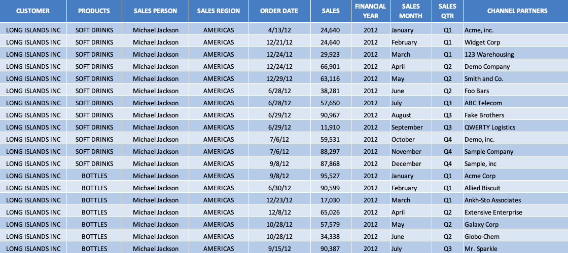
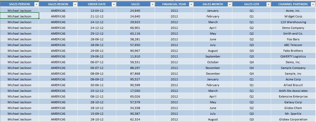
Here is our current Pivot Table setup:
STEP 1: Click anywhere on the data table.
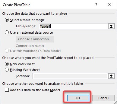
STEP 2: Go to Insert > PivotTable.
STEP 3: Place the Pivot Table in a New or Existing Worksheet and click OK.
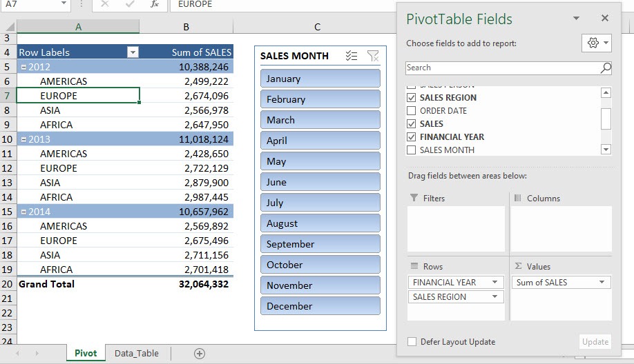
STEP 4: Drag and drop the following:
- Financial Year and Sales Region in Rows field
- Sum of Sales in Values field
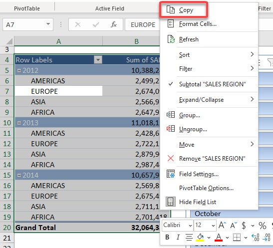
STEP 5: Select any cell inside the Pivot Table and go to PivotTable Analyze > Select > Entire PivotTable
STEP 6: Right-click and select Copy
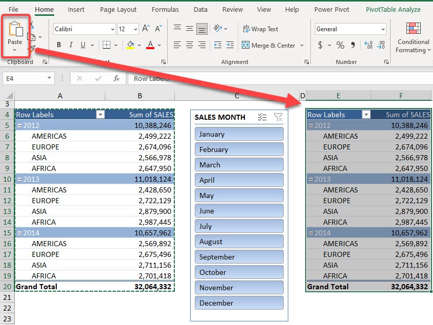
STEP 7: Pick an empty space and select Home > Clipboard > Paste
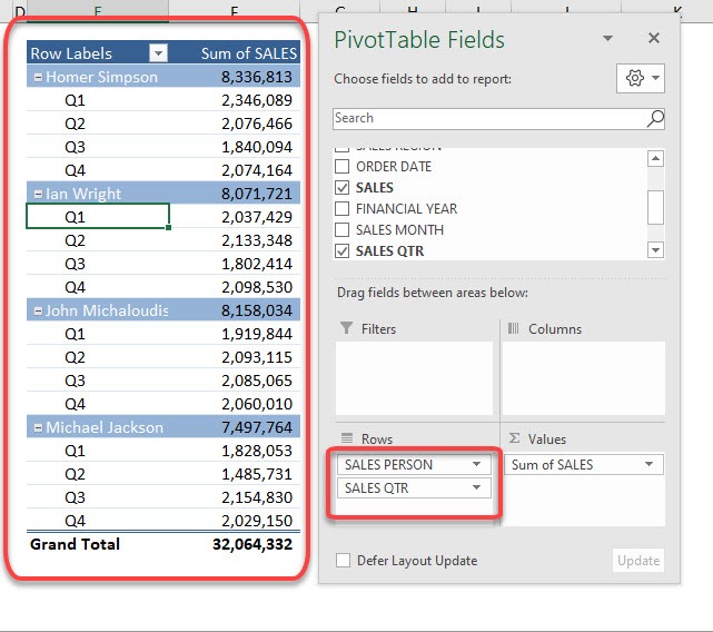
STEP 8: Now set up the second Pivot Table by placing inside Rows: SALES PERSON and SALES QTR
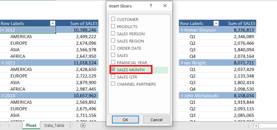
STEP 9: Click anywhere on the PivotTable, go to PivotTable Analyze > Insert Slicer.
STEP 10: Select Sales Month and click OK.
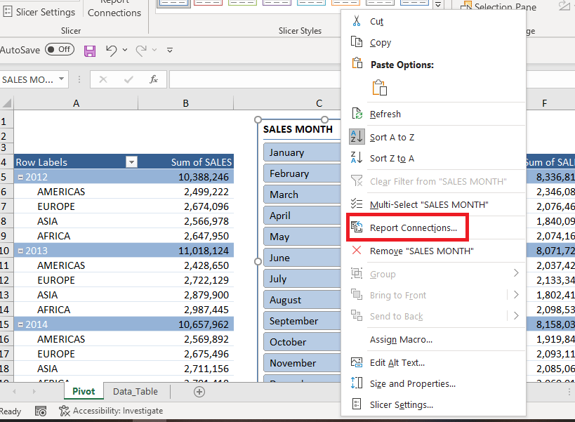
STEP 11: Right-click on the slicer and select Report Connections…
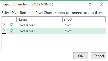
STEP 12: Select both the Pivot Tables and click OK.
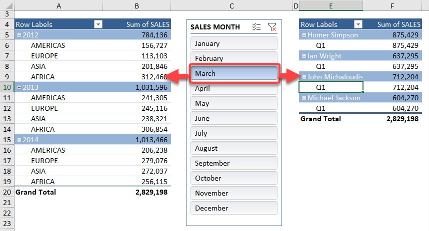
Now try it out! Click on March in your slicer and both pivot tables are updated at the same time!
You can choose the Report Connections options to link slicer to multiple pivot tables at once and use a single slicer to operate the pivot tables. This will make your report hassle-free and not messy.
Click here to learn more about Pivot Table Slicers!
Make sure to download our FREE PDF on the 333 Excel keyboard Shortcuts here:
Bryan
Bryan is a best-selling book author of the 101 Excel Series paperback books.
