Have you gotten overwhelmed with the amount of Tables whenever you used Power Pivot?
As I got accustomed to Power Pivot, my data model expanded and the number of relationships connecting these Tables together grew to a larger amount.
Fortunately, Power Pivot has the Diagram View feature, which gives you a birds eye view of your entire data model.
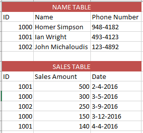
What we will focus on is a simple example of two Excel Tables: a Name Table and a Sales Table.
The crucial thing here is the relationship between these two tables. The ID column of the Sales Table related to the ID column of the Name Table.
You can see that each employee is uniquely identified by the ID number, which is also used in the Sales Table.
To make this example easy to understand, we have already linked these Tables to our Data Model, and we have already setup the necessary relationship between these two Tables.
*** You can view the exact step-by-step tutorial of how this was done here: Linking Excel Tables in Power Pivot.
Now you can download the prepared workbook and follow the steps to see how you too can use the Diagram View easily:
STEP 1: Open the Power Pivot Window. Go to Power Pivot > Manage.
(For Excel 2010, go to PowerPivot > PowerPivot Window)
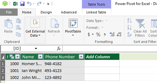
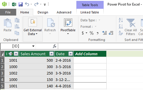
STEP 2: This will open Power Pivot Window. Your two Tables will already be loaded there.
Names Sheet:
Sales Sheet:
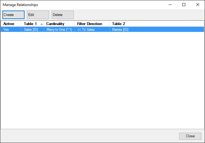
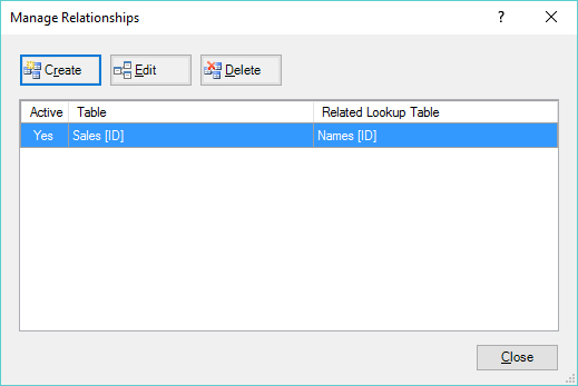
STEP 3: Go to Design > Manage Relationship.
The Relationship between the Sales Table and Name Table should be there:
EXCEL 2016 VIEW:
EXCEL 2013 & 2010 VIEW:
Close out of this.
STEP 4: Go to Home> Diagram View.
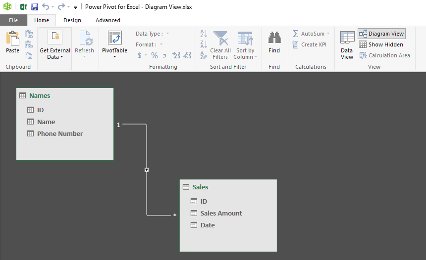
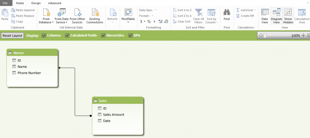
You are now shown an easy to read Diagram representing your Data Model and its relationships:
EXCEL 2016 VIEW:
EXCEL 2010 & 2013 VIEW:
Bryan
Bryan is a best-selling book author of the 101 Excel Series paperback books.
