What if you want to VLOOKUP multiple columns at once?
You can use Excel VLOOKUP multiple columns by using an Array Formula!
Without further ado let’s dive into these topics and understand how to use VLOOKUP for multiple columns!
As this is an array formula, to make it work we simply need to press CTRL+SHIFT+ENTER at the end of the formula. A very powerful feature for any serious analyst!” player-type=”default” override-embed=”default”]
Table of Contents
Excel VLOOKUP Multiple Columns Syntax
What does it do?
Searches for a value in the first column of a table array and returns the sum of values in the same row from other columns (to the right) in the table array.
Formula breakdown:
{=SUM(VLOOKUP(lookup_value, table_array, {col_index_num1,col_index_num2}, [range_lookup]))}
What it means:
{=SUM(VLOOKUP(this value, in this list, {and sum the value in this column, with the value in this column}, Exact Match/FALSE/0]))}
Now that you are familiar with the syntax let’s look at an example of how to use Excel VLOOKUP multiple columns!
Return Multiple Values
One of the downsides of using VLOOKUP is that it can return value from a single column only.
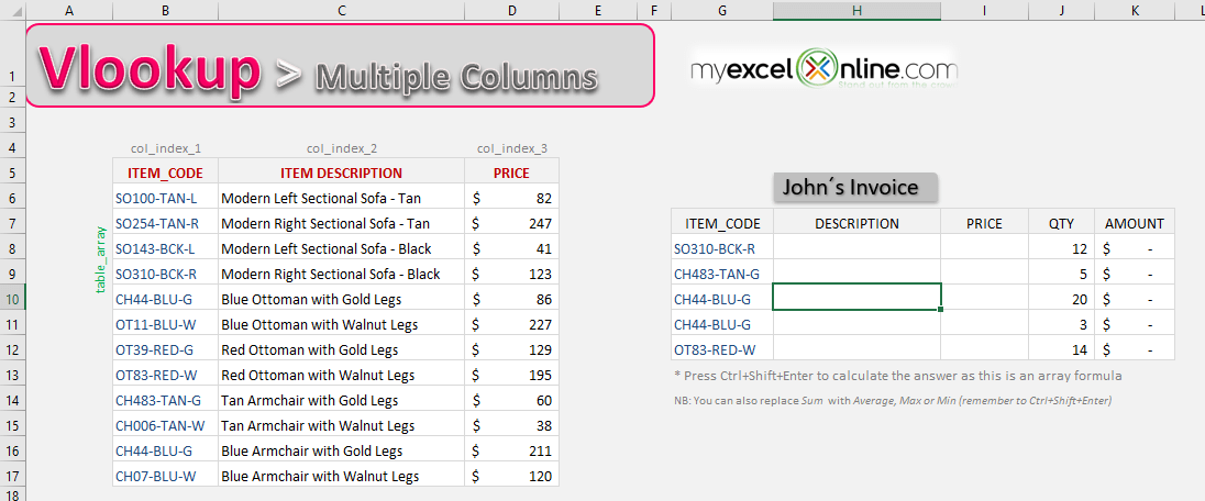
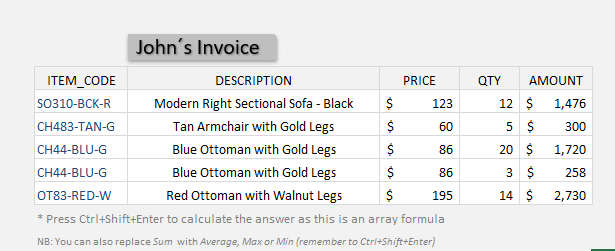
In this example, we want to find a match for both Item Description and Price. But it won’t be possible to use the basic VLOOKUP syntax.
You can modify the VLOOKUP formula with an array formula and extract both description and price by matching the item code!
Follow the step-by-step tutorial on how to VLOOKUP for multiple sheets with example and download this Excel workbook to practice along:
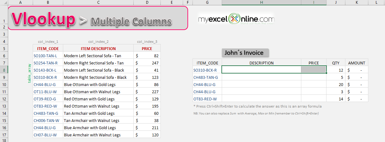
STEP 1: Select the cells (H8 and I8) where you want to insert the values from multiple columns.
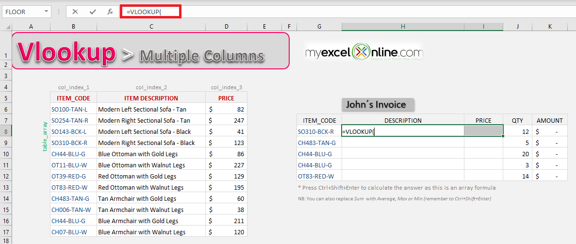
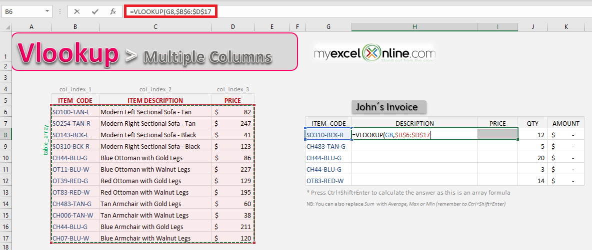
STEP 2: We need to enter the VLOOKUP function in the selected cell:
=VLOOKUP(
STEP 3: We need to enter the first argument – Lookup_value
What is the value to be looked up?
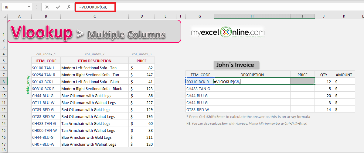
Select the cell that contains the item name, which is cell G8.
=VLOOKUP(G8,
STEP 4: We need to enter the second argument – Table_array
Where is the list of data?
Select the Inventory table, as that is where our formula is going to get both description and price for different item codes.
Make sure you freeze the range by pressing F4!
=VLOOKUP(G15,$B$6:$D$17,
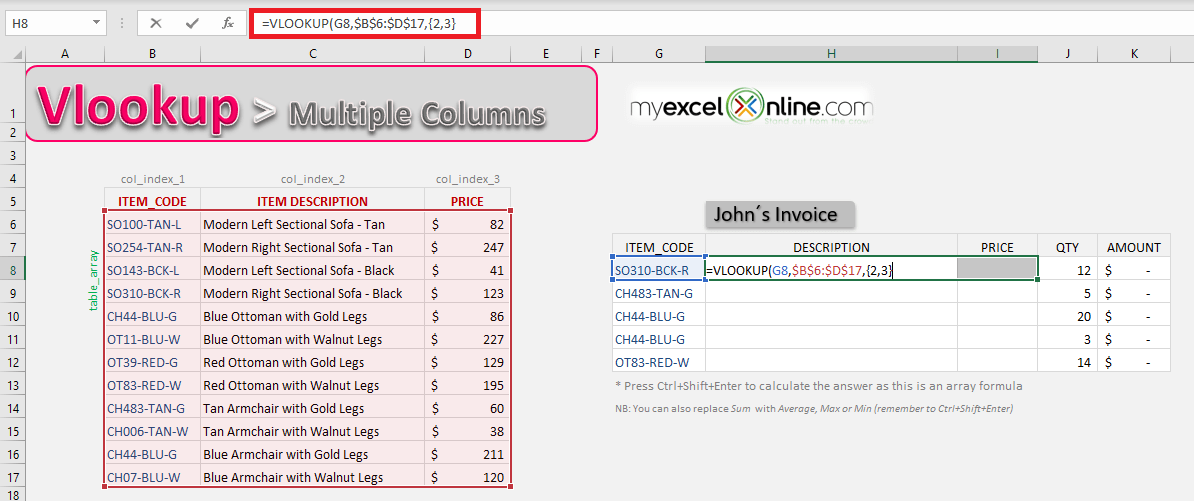
STEP 5: We need to enter the third argument – {Col_index_num1, Col_index_num2}
Which columns in the table_array contain the data you want to return?
We want to get the description and price. So that will be columns 2 and 3.
=VLOOKUP(G8, $B$6:$D$17, {2,3},
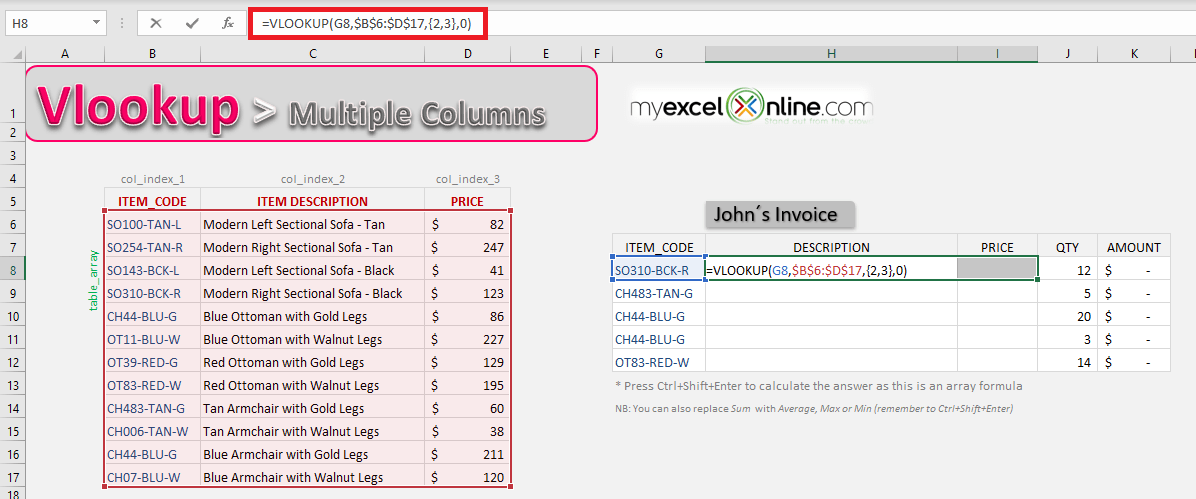
STEP 6: We need to enter the fourth argument – [Range_lookup]
Would it be an approximate match?
Set this to FALSE or 0 as we want an exact match for the Item code.
=VLOOKUP(G8, $B$6:$D$17, {2,3}, 0)
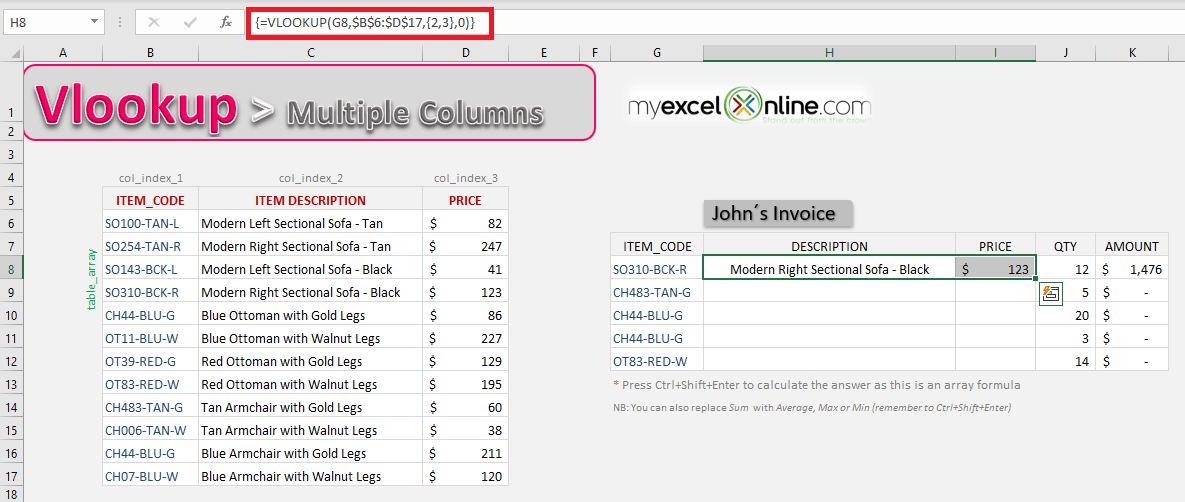
STEP 7: Press Ctrl + Shift + Enter at the end of the formula to change it into an array function.
Copy-Paste this formula for the remaining item codes mentioned in the Invoice!
Return Sum of Multiple Values
The VLOOKUP function can be combined with other functions such as the Sum, Max, or Average to calculate values in multiple columns. As this is an array formula, to make it work we simply need to press CTRL+SHIFT+ENTER at the end of the formula. A very powerful feature for any serious analyst!
See how easy it is to implement in less than 1 minute with this VLOOKUP for multiple columns example!
Want to learn more about how to use VLOOKUP to Sum Multiple Columns?
*** Watch our video above and step by step guide below on Excel VLOOKUP multiple columns with a free downloadable Excel workbook to practice ***
We want to get the total number of units for Laptop (16,700 + 18,700 units).
STEP 1: We need to enter the VLOOKUP function in a blank cell:
=VLOOKUP(
STEP 2: The VLOOKUP arguments:
Lookup_value
What is the value to be looked up?
Select the cell that contains the item name, which is Laptop.
=VLOOKUP(G15,
Table_array
Where is the list of data?
Select the Units Sold table, as that is where our formula is going to get the unit numbers.
=VLOOKUP(G15, B14:D17,
{Col_index_num1, Col_index_num2}
Which columns in the table_array contain the data you want to return?
We want to get the unit numbers of Years 2013 and 2014. So that will be columns 2 and 3.
=VLOOKUP(G15, B14:D17, {2,3},
[Range_lookup]
Would it be an approximate match?
Set this to FALSE as we want an exact match for Laptop.
=VLOOKUP(G15, B14:D17, {2,3}, FALSE)
STEP 3: Now wrap the formula with the SUM formula as we want to get the total number of sold units for Laptop.
=SUM(VLOOKUP(G15, B14:D17, {2,3}, FALSE))
Ensure you are pressing CTRL+SHIFT+ENTER as we want to calculate this as an array formula.
Do the exact same formula for Max Units and Average Units, by changing the SUM Formula with the MAX Formula and Average Formula respectively.
Conclusion
This completes our tutorial on how to use VLOOKUP to return values from multiple columns at once!
You can learn more about VLOOKUP basics, VLOOKUP with multiple criteria, and VLOOKUP in multiple sheets.
John Michaloudis is a former accountant and finance analyst at General Electric, a Microsoft MVP since 2020, an Amazon #1 bestselling author of 4 Microsoft Excel books and teacher of Microsoft Excel & Office over at his flagship Academy Online Course.
