‘VLOOKUP’ is now so common that everyone who has ever been working with Excel has heard of it.
Not necessarily because they know how to use it, but because some savvy Excel-user always talks about it at the office.
Advanced users have seen the use of Excel VLOOKUP multiple criteria to what the function is looking for. So if they would be searching for a ‘Nate Harris’ in an employee database, they would not want to search the entire database.
Instead, they would want to search for ‘Nate Harris’ but only in the ‘Sales-department’ of the company. This means that they would have two criteria for the search (‘Nate Harris’ and ‘Sales-department’).
By default, ‘VLOOKUP’ cannot help with a two-criteria (or more) lookup. It is customary to change to the more flexible combination of functions, ‘INDEX’ and ‘MATCH’ and turning the formula into an array formula. However, this is not as easy and intuitive as using a simple ‘VLOOKUP’.
In this article, I will guide you to how you can actually create an Excel VLOOKUP multiple criteria. It is an alteration of the typical way of using ‘VLOOKUP’ and is as intuitive as it is easy to use. But before you read on you should really know how to use ‘VLOOKUP’ the “normal” way.
Want to know how to use Excel VLOOKUP Multiple Criteria?
*** Watch our video and step by step guide below with a free downloadable Excel workbook to practice ***
Follow the step-by-step tutorial on how to VLOOKUP for multiple sheets with example and download this Excel workbook to practice along:
Download workbookVlookup-with-multiple-criteria.xlsx
The general idea
The basics of using VLOOKUP with multiple criteria scenario is that you will concatenate the different criteria so you can use them as a single lookup value.
The concatenation will in this example be done with the ampersand (&). That means that before we can go any further in the lookup, we need to conjure up a helper column that joins the ‘Table_arrays’.
The helper column
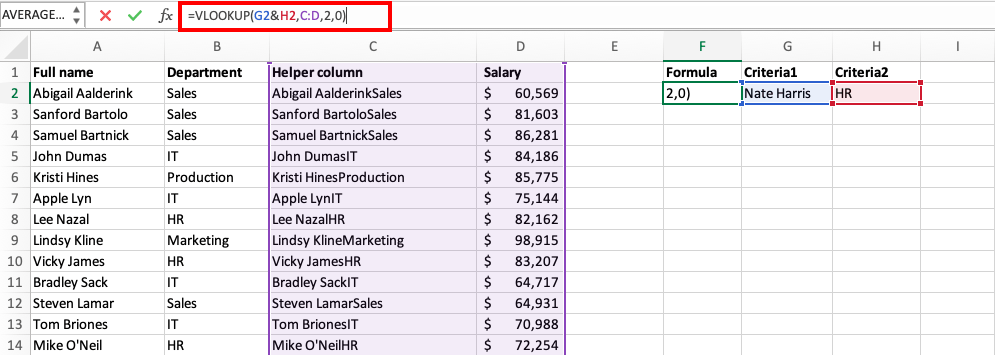
In this example, and in the sample file, we need to make a separate column that conjoins the data from the ‘Employee’ column and the ‘Department’ column. Take a look at the screenshot below.
Insert a column after column B and name it whatever you want in cell C1.
Enter the following formula into cell C2 and copy it down to the rest of the rows in the data.
=A2&B2
In short: The syntax of VLOOKUP
The things you need to put into a VLOOKUP formula to make it work (also called the syntax) is quite straightforward.
Follow the steps below:
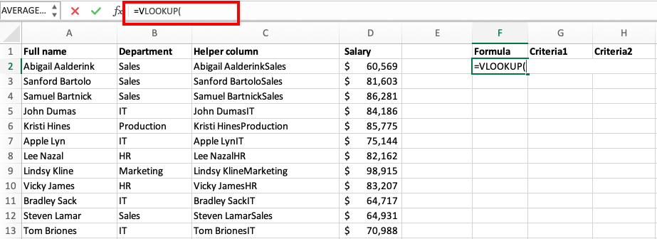
STEP 1: We enter the VLOOKUP function in the blank cell where we need to extract the data
=VLOOKUP(
STEP 2: Enter the first argument – lookup_value
The ‘lookup_value’ is what you are looking for, but not what you want as a result.
This is often a thing you already know, for example, the name of the employee (column A) and his department (column B), while the thing you don’t know (in this case) is the salary (column C).
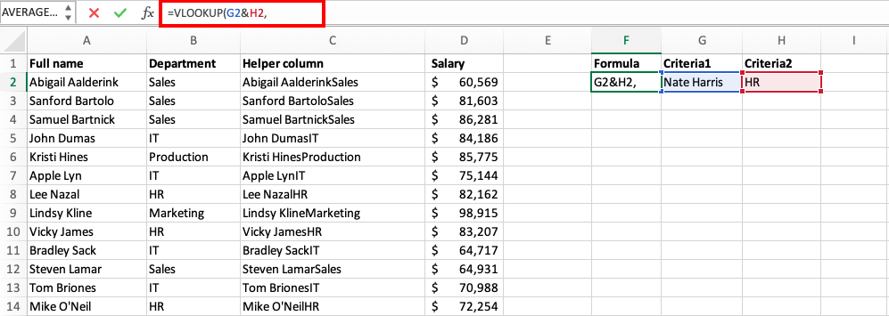
Creating an Excel VLOOKUP multiple criteria is to change the lookup value in the function. The lookup value should be a concatenation of the two criteria you want to include in the VLOOKUP.
Let us put the VLOOKUP formula in F2, the first criteria in G2 and the second criteria in H2. The lookup value of the VLOOKUP should be: G2&H2.
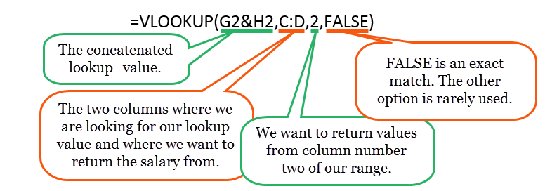
=VLOOKUP(G2&H2,
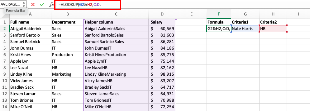
STEP 3: Enter the second argument – table_array
The ‘table_array’ is the area where you are looking for the data.
If you were using a “normal” ‘VLOOKUP’ it would be column A through C. Because of the helper column the range we must use in this case is column C through D.
=VLOOKUP(G2&H2,C:D,
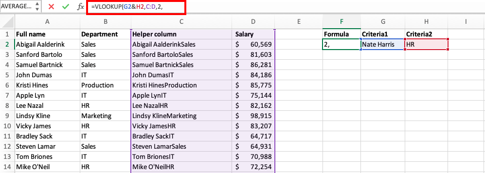
STEP 4: Enter the third argument – col_index_number
The ‘col_index_number’ tells which column you want to return the result from.
There are two columns in our ‘table_array’ and we want to return the salary, which is located in column D (the second column of our ‘table_array’). This number should be 2 in our example.
=VLOOKUP(G2&H2,C:D,2,
STEP 5: Enter the fourth argument – [range_lookup]
The [range_lookup] is simply a ‘TRUE’ or ’FALSE’ that tells Excel if we want to use an approximate or exact match for our lookup.
In the article on ‘VLOOKUP’, I referred to before you can read all about this. In this example, we just write ‘FALSE’ for this parameter of the syntax.
=VLOOKUP(G2&H2,C:D,2,0)
The final formula looks like this:
This completes our tutorial on how to create Excel VLOOKUP multiple criteria!
You’re done already!
Using VLOOKUP with multiple conditions is very easy (I told you!). Now you can change the criteria in cell G2 and H2 to test out your newly created multi-criteria lookup tool.
If you want to take your lookup skills even further, you should read here!
Guest Blog Post By:
Kasper Langmann from Spreadsheeto.com
Further Learning:
- XLOOKUP vs VLOOKUP: Top 5 Comparison of Excel Lookup Functions
- Why VLOOKUP not working in Excel – Top 5 Problems with Solutions
- 2 Easy Methods on How to Use XLOOKUP with Multiple Criteria
Make sure to download our FREE PDF on the 333 Excel keyboard Shortcuts here:
Bryan
Bryan is a best-selling book author of the 101 Excel Series paperback books.


