Ever wanted to lookup values in Excel? Which of the following Excel function did you use:
The dynamic one – VLOOKUP? The horizontal one – HLOOKUP? The complicated one – INDEX MATCH?
Even though the above Excel functions can get the job done, they come with their own limitations. The solution to this is to use the brand new Excel function introduced in Microsoft 365 – XLOOKUP!
If you are using any of the older versions of Excel (2010, 2013, 2016, 2019) you won’t be able to use this function.
XLOOKUP is a versatile and outstanding replacement for the above-mentioned Excel functions. It allows you to quickly lookup values in a data set (just like VLOOKUP Excel) with additional flexibility and advantages like:
- It can lookup data to the right or left of the lookup values.
- It looks for an exact match by default. You do not have to enter an additional argument for it.
- It allows you to provide a custom value or text if your search result is not found.
- It can perform a partial match lookup using wildcards.
- It can search for values both horizontally and vertically.
- It can return a range instead of a single value which spills out the results.
- It allows you to find the last occurrence in your data.
In this article, you will be provided a detailed guide on the following:
Table of Contents
Let’s look at each one of these points in detail!
XLOOKUP – An Introduction
What does it do?
Excel XLOOKUP can be used to search an array for a specific value and returns the value in the same row from another array.
- It can search the value both horizontally and vertically,
- Perform an exact or approximate match,
- Use wildcards,
- Return a custom text when no result is found,
- Doesn’t even have the restriction of the return array to be on the right of the lookup array.
Isn’t that AMAZING? It is a power-packed function with so many advantages!
Formula breakdown:
=XLOOKUP (lookup_value, lookup_array, return_array, [if_not_found], [match_mode], [search_mode])
where:
- lookup_value – the value you want to search;
- lookup_array – the range or array where you want to search the value;
- return_array – the range or array from which you want the result;
- [if_not_found] – the value you want to display if there are no results found;
- [match_mode]
- 0 – Exact Match (if no result found, then error)
- -1 – Exact or next smaller (if no result found, then the next smaller value will be displayed)
- 1 – Exact or next larger (if no result found, then the next larger value will be displayed)
- 2 – Wildcards
- [search_mode]
- 1 – to search from first
- -1 – to search from last
- 2 – binary search ascending
- -2 – binary search descending
Follow the step-by-step tutorial below and make sure to download the Excel workbook to follow along:
Now that you are comfortable with the syntax of this incredible function, let’s dive into a few examples to understand how to use Excel XLOOKUP!
How to use XLOOKUP in Excel?
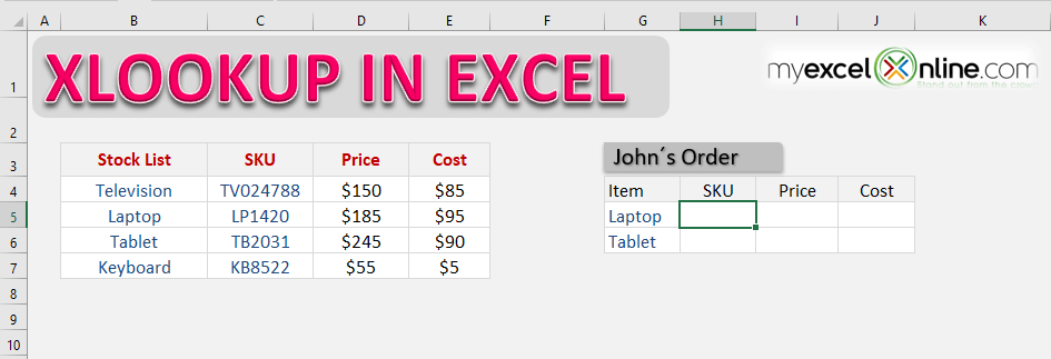
In this example below, there are two tables:
- Stocklist containing the product’s SKU, name, price, and cost.
- Orders Table with its quantity mentioned
You want to extract the price of the products from the stock list table using XLOOKUP.
STEP 1: We need to enter the XLOOKUP function in a blank cell
=XLOOKUP(
STEP 2:Enter the first XLOOKUP argument – Lookup_value (product’s SKU that you are looking for)
=XLOOKUP(H10,
STEP 3: Enter the second XLOOKUP argument – Lookup_array (the array that contains all product SKUs)
=XLOOKUP(H10,$E$9:$E$12
Ensure that you press F4 so that you can lock the table range
STEP 4: Enter the third XLOOKUP argument – return_array (the array that contains price)
=XLOOKUP(H10,$E$9:$E$12,$C$9:$C$12)
As you will see, Excel has pulled the price of the SKU LP1411 from the stock list and provided the result ($185) in the cell.
Apply the same formula to the rest of the cells by dragging the lower right corner downwards.
What if you are trying to search for a product name that is not available in the stock list table?
Excel will provide you with an error!
Instead of showing this error, you can add a custom text (say, No Product Found) to display!
To do that, simply can add the fourth optional argument of XLOOKUP function – [if_not_found]
=XLOOKUP(H10,$E$9:$E$12,$C$9:$C$12,“No Product Found”)
This was a basic example of how to use XLOOKUP in Excel. Let’s explore the advanced uses of this function in detail!
Approximate Match
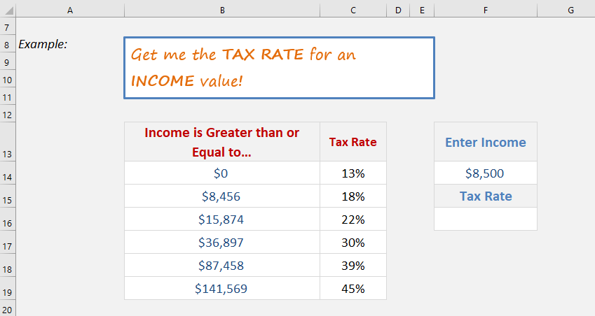
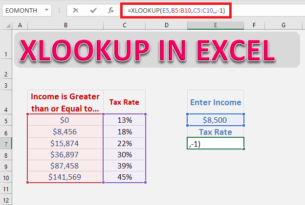
In this example, Excel will look for the income entered in cell F14 and find the matching tax rate from column C.
Instead of looking for an exact match, it will now look for an approximate match i.e. if an exact match is not found it will look for the next smaller or larger item based on the input provided.
If the income is greater than or equal to $0, the tax rate will be 13%. Similarly, if the income is greater than or equal to $8,456, the tax rate will be 18%, and so on.
So, let’s use this function to determine the tax rate for the income amount mentioned in cell F14.
=XLOOKUP (lookup_value, lookup_array, return_array, [if_not_found], [match_mode], [search_mode])
Here, the three permanent arguments and one optional argument [match_mode] will be used. You can ignore arguments – [if_not_found] and [search_mode] for this example.
Follow the step-by-step tutorial below to perform an approximate match using the XLOOKUP function:
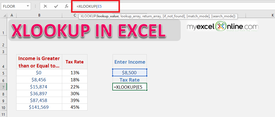
STEP 1: Enter the first argument lookup_value i.e. the income amount mentioned in cell E5.
=XLOOKUP(E5
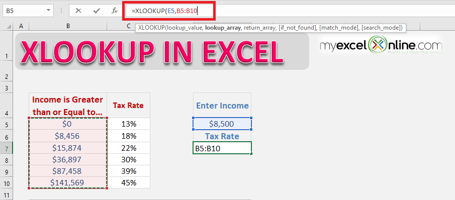
STEP 2:Enter the lookup_array i.e. the range containing income range (B5: B10).
=XLOOKUP(E5,B5:B10
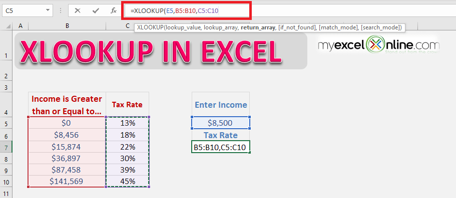
STEP 3:Enter the return_array
=XLOOKUP(E5,B5:B10,C5:C10
STEP 4: Enter the 5th argument[match_mode]. The accepted values for this argument are:
- 0 – Exact Match (if no result found, then error)
- -1 – Exact or next smaller (if no result found, then the next smaller value will be displayed)
- 1 – Exact or next larger (if no result found, then the next larger value will be displayed)
- 2 – Wildcards
In this example, the value will be -1.
=XLOOKUP(E5,B5:B10,C5:C10,,-1)
(Ignore the 4th argument)
Below is the formula that should be used:
=XLOOKUP(E5,B5:B10,C5:C10,,-1)
As you know this function will perform an exact match by default, you need to use the optional part of the function – [match_mode]. So, if Excel fails to find an exact match, it will look for the next smaller income range mentioned in the table.
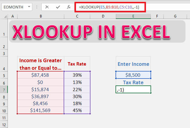
One of the advantages of using this function over Excel VLOOKUP for an approximate match is that you do not need to sort the data in ascending order. Excel will do that on its own!
In the example below, you will see that the data is not arranged in ascending order.
You can use the same formula in randomly arranged data and Excel will provide you with the same (correct) result.
Horizontal Lookup
The syntax for performing a horizontal lookup using XLOOKUP is the same as for vertical lookup.
You just need to provide Excel with the lookup and return an array, the table’s orientation is irrelevant to the XLOOKUP function.
In this example, the product name is displayed on Row 5 and the price is displayed on Row 6. You need to perform a horizontal lookup to get your results.
STEP 1:Enter the lookup value i.e. the product name mentioned in cell H6.
=XLOOKUP(H6
STEP 2:Enter the lookup array i.e. the array containing the product name.
=XLOOKUP(H6,$C$5:$F$5
STEP 3:Enter the return array i.e. the array containing prices of the product.
=XLOOKUP(H6,$C$5:$F$5,$C$6:$F$6)
It’s that easy to do a horizontal lookup using the new XLOOKUP function in Excel!
Return a Range instead of Value
Excel XLOOKUP has the ability to return multiple values instead of just one for a correct match. It can be done without making any change in the syntax, simply input the entire range in the function instead of just a single column or row.
In this example, we want to retrieve all the details related to the product name mentioned in cell G5.
STEP 1: Select the cell containing the lookup value.
=XLOOKUP(G5
STEP 2: Select the range containing the product list.
=XLOOKUP(G5,$B$4:$B$7
STEP 3: Select the entire range containing columns for SKU, price, and cost.
=XLOOKUP(G5,$B$4:$B$7,$C$4:$E$7)
Excel will extract or “spill” all the values with the help of the XLOOKUP formula!
Using Wildcards
Xlookup in Excel allows you to search for a partial match using wildcards characters like: * ? ~
This can be done using Excel VLOOKUP as well. But the problem arises when you are actually trying to search the wildcard character itself in the data.
For XLOOKUP, you can use wildcards in the lookup_value argument and specify that in the [match_mode] argument. Enter 2 as the match_mode value to let Excel know that you are trying to do a partial match.
The three wildcards in Excel are:
- Asterisk mark (*) represents any number of characters. For example, Jo* could mean Joanne, John, Joe, etc.
- Question mark (?) represents one character. For example, Jo?n could mean John, Joan, etc.
- Tilde (~) can be used when you want the asterisk or question mark to not be a wildcard. Simply place a tilde just before * or ?.
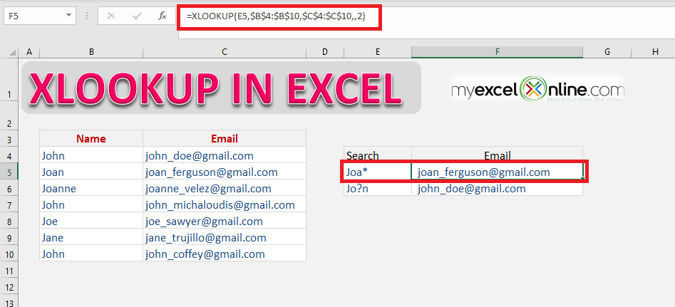
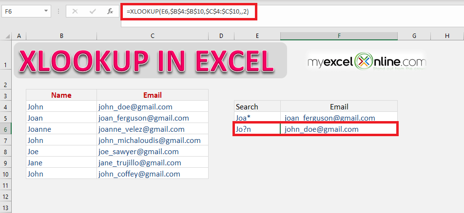
In these examples below, you can use wildcard characters (* or ?) to search for a partial match and return the corresponding email address.
Joa* will search for the first match starting with Joa and any number of characters after that (Joan) and return the corresponding email address ([email protected]).
=XLOOKUP(E5,$B$4:$B$10,$C$4:$C$10,,2)
Jo?n will search for the first match starting with Jo followed by one character and then n (John) and return the corresponding email address ([email protected]).
=XLOOKUP(E6,$B$4:$B$10,$C$4:$C$10,,2)
Search from bottom to top
In this example, we will search the value from bottom to top instead of the default direction (top to bottom). This can be achieved by using the 6th argument of the function – [search_mode].
It is an amazing feature if you wish to find the last occurrence of something in your data. Let’s dive into this XLOOKUP example to learn how.
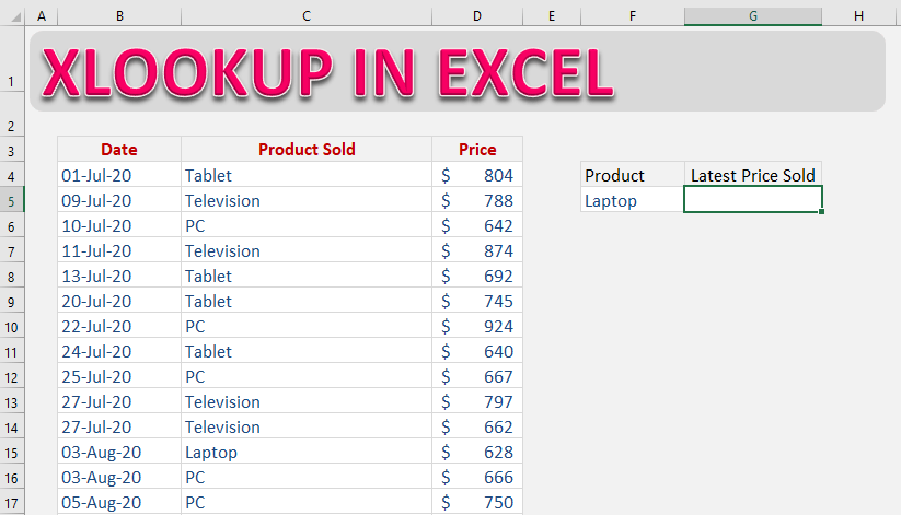
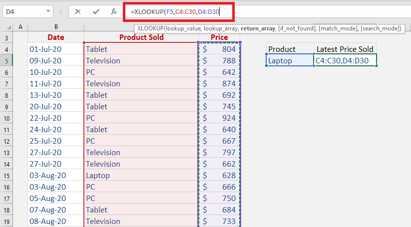
In this example, you have sales data with the Sales date, Product name and Price mentioned. You have to find out the latest price at which a particular product was sold.
Follow the step-by-step tutorial to search value from bottom to top:
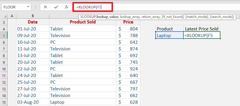
STEP 1: Enter the lookup value i.e. the product name mentioned in cell F5.
=XLOOKUP(F5
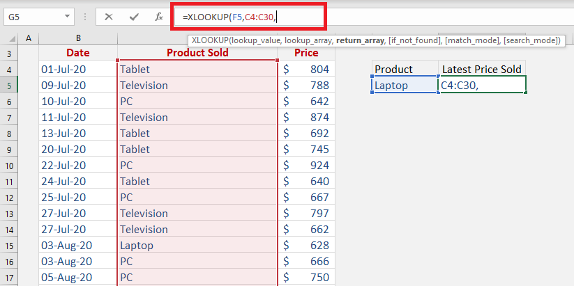
STEP 2:Enter the lookup array i.e. the array containing the product name.
=XLOOKUP(F5,C4:C30
STEP 3:Enter the return array i.e. the array containing prices of the product.
=XLOOKUP(F5,C4:C30,D4:D30
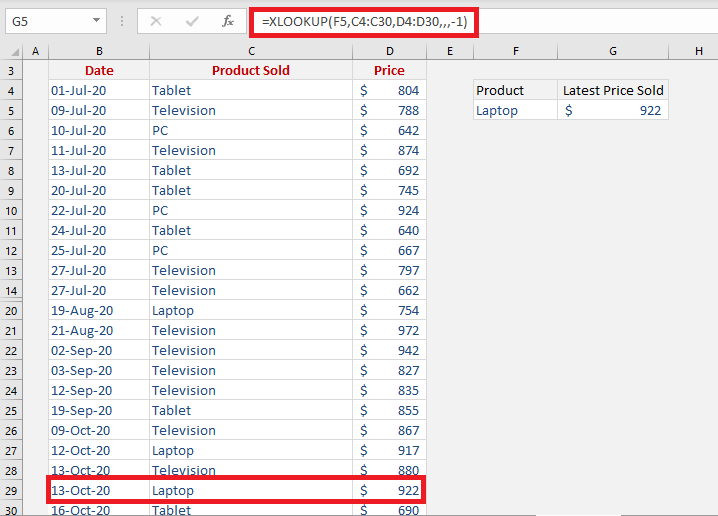
STEP 4:Enter the 6th argument [search_mode]. It will be -1 for this example as you want to search from bottom to top.
=XLOOKUP(F5,C4:C30,D4:D30,,,-1)
Excel will start the search from the bottom and the first match will be produced as a result!
Conclusion
XLOOKUP is the latest and outstanding addition to the Excel lookup family. It can search for a value and return the matching result, similar to the Excel VLOOKUP.
But that’s not it!
There are several reasons why this new XLOOKUP function is better:
- It can lookup data to the right or left of the lookup values.
- It looks for an exact match by default. You do not have to enter an additional argument for it.
- It allows you to provide a custom value or text if your search result is not found.
- It can perform a partial match lookup using wildcards.
- It can search for values both horizontally and vertically.
- It can return a range instead of a single value which spills out the results.
- It allows you to find the last occurrence in your data.
This AWESOME function is available for Microsoft 365 users only. Click here to purchase it! You can also go through the Microsoft tutorial on XLOOKUP by clicking here!
Further Learning:
- XLOOKUP vs VLOOKUP: Top 5 Comparison of Excel Lookup Functions
- 2 Easy Methods on How to Use XLOOKUP with Multiple Criteria
- Top 11 Examples of Using XLOOKUP in Excel – The Ultimate Guide
Make sure to download our FREE PDF on the 333 Excel keyboard Shortcuts here:
You can learn more about how to use Excel by viewing our FREE Excel webinar training on Formulas, Pivot Tables, Power Query, and Macros & VBA!
John Michaloudis is a former accountant and finance analyst at General Electric, a Microsoft MVP since 2020, an Amazon #1 bestselling author of 4 Microsoft Excel books and teacher of Microsoft Excel & Office over at his flagship Academy Online Course.


